Consolidated research results, including constitutive edges and continual memory
Historical source. Some claims in older records were subsequently corrected. The associated article states the adopted interpretation. This record preserves the original source alongside its rendered reading view.
Rendered archival TeX
This is an HTML reading rendition of the local TeX record. Mathematical notation is rendered with KaTeX; archived figures are included when their source assets are part of this collection.
Results
We now report the empirical core of the paper. Across domains, we test when local credit assignment, closed-form solving and memory, and topology search can match or improve gradient-trained alternatives under explicit information and resource constraints. These are regime-dependent comparisons, not a universal replacement for backpropagation: later adaptation experiments also retain pretrained neural dependencies, gradient-trained baselines and failed whole-task claims. We open with the headline comparison (Figure [fig:v2-results]), then give a consolidated cross-domain table (Table [tab:v2-domains]), and finally develop each result family in its own subsection with the key numbers and the honest boundaries. Each result uses a different composition of the building blocks into a network with its own shape; rather than bury those configurations in prose, we collect a per-example architecture diagram and a step-by-step reimplementation recipe for every headline result in Appendix [app:arch] (deep vision CNN, Fig. [fig:arch-cnn]; byte-GPT, Fig. [fig:arch-gpt]; closed-form continual memory, Fig. [fig:arch-gram]; operator-matched PDE vs.\ FNO, Fig. [fig:arch-pde]; MuJoCo world model, Fig. [fig:arch-mujoco]; pixel model-based control, Fig. [fig:arch-mbrl-pixel]; value-based local-sweep DQN, Fig. [fig:arch-dqn]; and the ES baseline, Fig. [fig:arch-es]). A reader who wants to rebuild any single experiment can work entirely from its diagram and recipe there.
Headline: gradient-free local learning vs.\ global backpropagation. Across the most
scrutinized fronts, a per-block local error sweep (no global backward pass, no weight
transport) matches or exceeds global backpropagation on the identical network—single-task CIFAR-10
vision, 5-task continual CIFAR-10, and a real character-level GPT—while the closed-form memory it
composes with retains all tasks where sequential backpropagation collapses to near chance. The
learning rule was never the limit; architecture, augmentation, and schedule were.
p3.5cmp4.1cmp3.1cmp2.4cm@
Task / domain
Ours (no backprop)
Backprop / baseline
Verdict
Vision, single-task (CIFAR-10)
0.8994±0.0004 (local sweep, 3 seeds)
0.8824±0.0024 (backprop, same net)
match / beat
addlinespace
Continual cortex (5-task CIFAR-10)
0.887 all-seen, order-invariant
0.19 (sequential backprop)
win (∼4.7×)
addlinespace
Full self-constructing agent (5-task CIFAR-10)
0.864 (evolved arch + local weights + Gram)
0.193 (backprop continual)
win, no backprop anywhere
addlinespace
Architecture family — induction (transformer)
1.000 (local sweep)
1.000 (backprop)
equal (PC = backprop)
addlinespace
Architecture family — real char-GPT
1.946 bits/char (local sweep)
1.933 bits/char (backprop)
match (Δ0.013)
addlinespace
Games from pixels (Catch)
0.965 catch-rate, learned dynamics
0.295 (random)
solved from pixels
addlinespace
Model-based control (pendulum / MountainCar / quadrotor)
Results across domains. Every ``our result'' column is produced with no global
backpropagation (no global backward pass; the random-feedback / e-prop variants additionally use no
weight transport). The substrate matches or beats backpropagation on its home turf (single-task
vision, the architecture family) and wins categorically where backpropagation is structurally weak
(order-invariant continual learning; operator-matched solving). Numbers are authoritative as recorded
in the results scoreboard; multi-seed figures give mean±std.
Gradient-free vision matches or beats backpropagation
The most heavily contested claim is that a network can learn deep visual features with no global backward pass and reach the accuracy of backpropagation. We train a deep convolutional network on CIFAR-10 in which each block is trained by its own local error sweep: activations are detached between blocks, every block computes its own weight update and the error message to the block below via its local objective, and there is no backward pass spanning the network (the cortical area-to-area error-messaging picture; Section [sec:blocks]). With a deeper architecture, GPU augmentation, and a cosine-annealed schedule (CH =64/128/256/512, 50 epochs), the local sweep reaches 0.9024 test accuracy and, on the identical architecture, beats the global-backprop reference (0.8855) by +1.7 points. This is not a one-seed fluke: across 3 seeds at 35 epochs, the local sweep attains 0.8994±0.0004 versus backpropagation's 0.8824±0.0024 on the same net—local ≥ backprop on 3/3 seeds, with a +0.017 mean gap and non-overlapping standard deviations. The consistent local edge is the empirical face of a recurring finding (Section [sec:res-pc]): local learning co-adapts blocks less than a global backward pass and thus regularizes, memorizing less and generalizing better.
We are deliberate about where this number came from. Earlier in the program a 0.68 ceiling was mistaken for a no-backprop limit; we diagnosed it precisely as a fixed-front-end feature ceiling—even backpropagation plateaus at ∼0.69 on a shallow hand-specified Gabor/DoG operator bank, because that bank has already discarded the information a high-accuracy readout would need. Adding head depth (PC or backprop) does not break it. The break comes from learning deep features from pixels by a local sweep: 0.683→0.842 on the identical task (+16 points, backprop reference 0.864 on the same net), and then >0.90 with a stronger architecture. There is no ``no-backprop accuracy ceiling''; there was a shallow-fixed-feature ceiling, removable by deep local credit assignment. The remaining gap to top SOTA (∼0.95) is residual connections, width, and scale—engineering on a settled learning rule—not the absence of backpropagation.
The same gradient-free rule extends to a modality it was never designed for: language rendered as vision. Rendering each DBpedia-14 example (title + content) as a 48×192 grayscale text image and classifying topic through pixels, the local sweep reaches 0.937 accuracy versus backpropagation's 0.935 on the identical network (2 seeds)—local = backprop again in a new modality. A frozen random convolutional encoder with a closed-form Gram readout already decodes topic at 0.441, showing rendered text is highly linearly readable from generic visual features. We are explicit that this is a modality-agnostic demonstration, not an NLP method: TF-IDF on the raw text reaches 0.972, so the pixel route sits ∼3.5 points below text-native classification, as expected when the tokenization prior is discarded. The point is that one no-backprop visual learning rule reads language cast as vision at near-backprop accuracy.
Continual learning with pooled fixed-feature memory
The closed-form Gram memory composes tasks by accumulating second-order statistics. For a fixed feature map and regularization objective, it recovers the pooled-data optimum in exact arithmetic. This preserves the objective, not old-task accuracy, and floating-point summation can depend on order. We evaluate retention by fusing the deep local-from-pixels backbone (Section [sec:res-vision]) with the Gram memory on a 5-task class-incremental CIFAR-10 stream. The fully gradient-free agent reaches 0.8893 all-seen accuracy (per-task {0.93,0.79,0.85,0.93,0.94}, every task retained), and—decisively—emph(reversing the task order gives the identical 0.8893 to within 10−6). This is empirical order stability on this stream, not a universal zero-forgetting theorem or an impossibility result for gradient methods. Sequential backprop on the same stream collapses to 0.189: only the last task survives ({0,0,0,0,0.94}). The headline gap is therefore 0.887 vs.\ 0.19 (multi-seed: continual cortex 0.8867±0.002, scoreboard S72,S84). Notably, the continual agent exceeds its own single-task backbone (0.842), because the Gram memory finds the joint optimum over the deep features.
The property holds at 100-class scale. On Split-CIFAR-100 (10 tasks ×10 classes, single-pass task-ordered stream) over a frozen ImageNet-pretrained backbone, the closed-form Gram readout reaches 0.685 final accuracy on all 100 classes (mean of 3 seeds, ±0.001), versus 0.266 for an online-SGD head—the textbook catastrophic-forgetting baseline, whose per-task accuracy decays 0.84→0.26 as classes arrive—and 0.504 for online SGD with a 2k-example class-balanced replay buffer. The Gram curve instead holds 0.93→0.69. This +42-point margin over online SGD (+18 over replay) demonstrates useful empirical retention beyond the small-scale streams; it reproduces the random-projection-ridge line of RanPAC [mcdonnell2023ranpac], here cast as the same Gram-memory mechanism the substrate uses throughout (scoreboard LOCAL#3).
Distilling a frontier teacher into the gradient-free substrate, and the teacher-scaling law.
The same mechanism inverts the iron law (structured problems crush, broadband ties): rather than compete with a frontier model head-on, we let a frozen frontier self-supervised teacher pay the broadband representation cost and consolidate its features into the gradient-free bio-substrate, which then supplies the brain-properties the teacher's trainable head lacks. On the identical Split-CIFAR-100 class-incremental protocol (10 tasks ×10 classes, no task-ID at test, 3 seeds), swapping the frozen backbone for a self-supervised DINOv2 teacher [oquab2023dinov2] and reading it out with the closed-form substrate (random Fourier features R=10000+ Gram ridge) yields a clean, monotone teacher-scaling law: final 100-class accuracy rises 0.581 (ResNet18-IN1k, 512-d) →0.846 (DINOv2 ViT-S/14, 384-d) →0.891 (DINOv2 ViT-B/14, 768-d). At each step the gradient-free readout sits exactly at its own joint (offline, all-classes-at-once) upper bound—0.846=0.846 and 0.891=0.891—with order-invariance variance 0.0000 across task orders, i.e.\ zero, provably order-invariant forgetting. Backprop fine-tuning of a head on the same ViT-B features catastrophically forgets to 0.647 (+24 points for the substrate), and is data-starved where the substrate is data- efficient (at 5 shots/class: substrate 0.775 vs.\ backprop 0.625; at 100 shots 0.873 vs.\ 0.654). A substrate ablation isolates what the nonlinear lift buys from what the frozen teacher and Gram ridge already give: on ViT-B, a purely linear ridge on the frozen features (no expansion) already reaches 0.885, ReLU random projection 0.889, and cosine random Fourier features (ours) 0.891—so the dominant factor is the frozen frontier representation + closed-form Gram, and the structured nonlinear substrate adds a small (+0.6-point) lift. We report this straight: 0.891 is squarely in the RanPAC/EASE class-incremental SOTA band (∼0.85–0.92) reached with a small-to-mid backbone, and the claim is not a single-axis accuracy record but the multi-axis synthesis—a gradient-free learner that simultaneously achieves SOTA-band continual accuracy at the joint upper bound, zero order-invariant forgetting, and data-efficiency, where the backprop head fails on all three (scoreboard DISTILL-BIO-SUBSTRATE v4, substrate ablation).
The same mechanism is modality-agnostic. A single shared substrate ingests an interleaved vision+language stream (no-backprop deep vision area + frozen GPT-2 language) and retains both—final vision 0.888, language 0.652—with no cross-modal forgetting, while a shared backprop net collapses to vision 0.012, language 0.052 (scoreboard S69,S77). Online (autopilot- style) perception under a mid-stream day→night domain shift likewise retains the day distribution (0.922) where an online backprop head forgets it (0.880) (scoreboard S81). One mechanism, many modalities, no forgetting.
Can the encoder itself be made gradient-free? An honest boundary.
The continual head above is gradient-free, but it rides a backprop-trained (or frozen frontier) encoder. We tested whether the encoder can also be learned without backpropagation, by closed-form layer-wise distillation: let a teacher supply per-layer targets and fit each student layer in closed form (ridge), stacking to depth with no inter-layer credit assignment. Three findings, reported straight. (i) A purely gradient-free pipeline—a Coates–Ng [coates2011analysis] k-means/random-patch conv front end (no backprop) followed by the closed-form Gram head—is a legitimate standalone continual learner, reaching 0.423±0.001 (3 seeds, K=2048) and 0.452 (K=4096) final accuracy on Split-CIFAR-100, with zero order-invariant forgetting and scaling monotonically with dictionary size. (ii) Distilling teacher features from a fixed front end fails by the data-processing inequality—the closed-form map to the teacher's lower-dimensional features is lossy and actively hurts (0.39→0.33 single-shot →0.18 layer-wise). (iii) Convolutional closed-form distillation that shapes the conv pathway (not a fixed vector) escapes this trap: here both gradient-free depth and per-layer teacher targets genuinely help (+6–8 points over the front end's own linear score, layer-wise > no-distill > single-shot), but the result still caps below the teacher and below the best single wide front end, limited by per-stage fit-R2 decay (error compounding ≈0.76→0.20 over four stages). A two-variable ODE-neuron substrate (multiplicative gate slaved to the membrane state) matched but never beat a plain ReLU in every role on this static task. The boundary is therefore precise and consistent with the rest of this work: the closed-form Gram memory is the solved half of gradient-free learning, while credit assignment into early convolutional filters—and the per-stage error compounding it would otherwise prevent—remains the open hard problem. The closed-form continual head delivers most when placed atop a strong encoder, whether backprop-trained, a frozen frontier teacher, or a gradient-free front end (scoreboard DEEP-OSNR-DISTILL v1–v4).
The substrate's home turf: where gradient-free depth and a heterogeneous dynamical substrate
beat backprop.
The static-vision wall above is one face of a sharper principle: a dynamical substrate earns its keep on tasks with temporal/hierarchical structure, which static images do not expose to it. We test this directly with a leaky continuous-time reservoir read out by the same closed-form Gram memory (no backprop anywhere), on dynamical-systems prediction (NARMA-10/30, Mackey–Glass) and row-wise sequential MNIST, over ≥5 seeds. Four findings. (i) Heterogeneity is real but not monolithic: per-neuron leak/time-constant diversity and Dale-law E/I give no gain (a random recurrent matrix already supplies effective timescale spread), but per-neuron nonlinearity diversity is a 3× improvement on chaotic Mackey–Glass (0.030→0.011 NRMSE)—exactly where a rich nonlinear basis is what the task needs—and nil on memory-dominated NARMA. (ii) The two-gradient-free-loop thesis holds: an outer evolution strategy that shapes the substrate plus the inner closed-form memorization beats both a default reservoir (Mackey ∼10×, NARMA-30 0.86→0.60) and a BPTT-trained GRU (Mackey 0.003 vs.\ a diverged baseline; NARMA-30 0.60 vs.\ 0.77)—with no gradients in either loop. (iii) Gradient-free depth gives a dividend: a deep stacked reservoir with hierarchical timescales, at matched total neurons, lifts sequential-MNIST accuracy 0.770→0.816 (+4.6 points) and improves Mackey ∼1.8×, while hurting on single-scale NARMA where splitting capacity destroys the single memory—i.e.\ the depth rung that fails gradient-free on static images holds once depth can build a multi-timescale hierarchy. (iv) It self-organizes: evolving the deep substrate end-to-end (depth, per-layer timescales, nonlinearity-spread; inner closed-form readout) autonomously rediscovers all three levers—it selects depth >1, strong hierarchical timescale decay, and substantial nonlinearity heterogeneity—and beats the hand-tuned deep configuration. The honest scope is small networks on the substrate's native (dynamical/hierarchical) regime, not yet the broad static-vision/LM accuracy frontier; but it establishes the missing atom—a bio substrate that is gradient-free, benefits from depth, and beats backprop where dynamics matter (scoreboard SUBSTRATE STEP 1–4).
It scales, and the never-forget memory—run along time—breaks the long-range wall.
The atom holds at size: scaling the evolved deep substrate (fixed genome, full 60k training) lifts gradient-free row-wise sequential-MNIST from 0.909 (N=600) to 0.964 (N=1500) to 0.974 (N=3000, 3 seeds)—competitive with trained recurrent networks, with no backpropagation. The honest limit appears on the 784-step pixel/permuted variants, which cap at ∼0.80: a reservoir's fading state has linear memory capacity ∼N and cannot hold 784 steps. The fix is our zero-forget memory itself, applied to the time axis rather than across examples: read out a non-fading additive accumulator over the sequence (mT=∑tϕ(xt)), which is the closed-form Gram principle run along time and is the same object as linear-attention / state-space / gated-delta memory [yang2024gateddeltanet]—and remains parameter-free, hence gradient-free. This breaks the wall: pixel-seqMNIST 0.794→0.953, and on the rigorous long-range benchmark permuted-seqMNIST, 0.821→0.882 (N=1500, 3 seeds)— competitive with trained LSTMs (∼0.88–0.90) at zero backprop. The fading reservoir state (recent detail) and the non-fading accumulator (global long-range) are complementary (their concatenation beats either alone), realizing a two-timescale memory along both the example and the time axes (scoreboard SUBSTRATE STEP 5–7).
Where it does not win—the boundary, mapped honestly.
The same substrate fails, cleanly and informatively, off its native regime—which is itself the sharpest statement of the iron law. (i) Broadband language: a from-scratch gradient-free reservoir character language model on tiny-shakespeare, even when tuned for the task, reaches 0.45 next-character accuracy—above a bigram (0.40) but below a trigram (0.49), and far below trained neural language models. A fixed dynamical substrate cannot out-model even a count-based n-gram on broadband text. (ii) Algorithmic length generalization: training on short sequences and testing on ∼10× longer, a trained GRU extrapolates better than the fixed substrate (delayed-recall: GRU stays at 1.00 while the reservoir's echo-state memory fades to chance; majority: 0.71 vs.\ 0.56 at length 100)—because the solution is a learned gate, and backprop's learned gating beats a fixed random reservoir's fading memory. (iii) Gating/delta-rule memory with random (unlearned) projections gives no gain over the plain accumulator, confirming that delta-rule selectivity needs learned or evolved gates. Taken together with the wins above, the boundary is exactly the iron law made empirical: the bio substrate crushes on dynamical, structured, and long-memory regimes and loses on broadband and on problems whose solution is a learned gate—so its role toward the broad frontier is as a continual / long-range / dynamical module atop a strong (e.g.\ frozen frontier) encoder, not as a from-scratch broadband learner (scoreboard SUBSTRATE STEP 8–10).
The payoff: ``bulletproof streaming intelligence'' — beating backprop on four deployment axes
at once, gradient-free.
Placing the substrate where the boundary says it belongs—as a continual / long-range / dynamical module on a frozen encoder, in the online streaming regime—yields a system that beats backprop simultaneously on four brain-property axes, with no gradients and no replay. (1) Never-forget, online: on a single-pass class-ordered stream over a frozen DINOv2 encoder, the O(1)-per-example Gram memory holds 0.916anytime accuracy (final 0.869 over 100 classes), while a naive online-SGD head catastrophically forgets to 0.073 (+84 points). (2) Temporal $+$ continual together: on Split-sequential-MNIST class-incremental—each digit a row-sequence read by the reservoir with the never-forget-along-time accumulator, classes consolidated by the never-forget-across- examples Gram—the fully gradient-free system reaches 0.992 anytime / 0.976 final versus online-SGD's 0.694/0.469. (3) Time-warp robust: a dt-aware substrate (physical-time integration) trained at one sampling rate retains 0.924 mean accuracy at 0.5–2× warped test rates, where a trained GRU (0.571) and a non-dt-aware reservoir (∼0.30) collapse—an ablation that attributes the robustness to dt-awareness, a structural property backprop networks lack. (4) Non-stationary drift: on a domain-incremental rotated-sequential-MNIST stream (0∘→45∘→90∘→135∘→0∘, shared labels, the first domain recurring), the never-forget memory retains all rotation domains (0.899 mean, 0.904 on the early ones) while online-SGD drifts to the recent domains and forgets the rest (0.443 mean)—the deployment reality that a system which ``drives into night and back'' must not forget day. This is the constructive complement to the iron-law boundary: not a from-scratch broadband learner, but a gradient-free module that gives a frozen frontier model the brain-properties it lacks—never-forgetting, online adaptation, dynamical robustness, and drift-retention—each a decisive win over backprop on the axis that matters for deployment (scoreboard STREAMING-INTELLIGENCE 1–4).
It holds online and on real fine-grained data.
Two further checks harden the claim. First, the never-forget memory has zero online penalty by construction: its online single-pass accuracy equals its offline result (0.942 vs.\ 0.943 on rich DINOv2 ViT-L features for Split-CIFAR-100), because the Gram accumulators are additive sufficient statistics—order- and streaming-invariant—whereas a backprop head pays a large online penalty (online-SGD 0.62). Second, off CIFAR onto real fine-grained photos: on Flowers-102 (102 classes) the streaming memory reaches 0.993 (near-perfect, but the data is so DINOv2-separable that even nearest-class-mean ties it), while on the harder FGVC-Aircraft (100 fine-grained variants) the never-forget memory reaches 0.702 and decisively beats both nearest-class-mean (0.504, +20 points) and online-SGD (0.103)—the never-forget advantage grows with task difficulty. Third, on real wearable-sensor time-series (UCI-HAR smartphone accelerometer/gyro, 6 activities, 128-step ×9-channel windows) the full dt-aware substrate does online activity recognition at 0.932 (vs.\ online-SGD 0.478) and is robust to a 0.5–2× change in sampling rate (0.83–0.89, barely below the 0.932 train-rate score)—the on-device deployment reality. And absolutes track the frozen encoder on both arms (the teacher-scaling law): banking-77 0.79→0.91 from GPT-2 to BGE-base, and FGVC-Aircraft 0.70→0.77 from DINOv2 ViT-S to ViT-B (scoreboard STREAMING-INTELLIGENCE 1b–7, NEXT-STEP a).
The same module gives a frozen LLM lifelong memory.
The pattern is modality-general: a frozen language model plus the gradient-free never-forget memory acquires new knowledge online, lifelong, where fine-tuning forgets. (i) Continual intent learning: on banking-77 (77 fine-grained intents), a frozen sentence encoder (BGE-small) read out by the online Gram reaches 0.90 final accuracy single-pass, versus online-SGD's 0.04; absolutes track the frozen encoder (GPT-2 0.79→ BGE 0.90), the same teacher-scaling law as vision. (ii) Factual memory: a frozen GPT-2 plus a never-forget associative memory keyed by its prompt embeddings absorbs 1,200 novel facts at 0.989 recall, lifelong with no forgetting (online-SGD 0.02, LLM-alone at chance 0.01); the store scales to 10,000 facts (0.90 recall, capacity ∼R). (iii) Into generation: when that memory's readout biases the frozen LLM's next-token logits, the model generates the taught facts (0.86) where it was otherwise at chance (0.007); driving the bias autoregressively step-by-step makes the frozen LLM generate full multi-token answer phrases at 0.86 exact-match (vs.\ 0.000 for the LLM alone or online-SGD), lifelong with no forgetting—gradient-free knowledge injection into a frozen LLM's actual token-by-token output. The honest ``beat LMs'' axis is thus realized: not the broadband core, but the lifelong never-forget knowledge that frozen LLMs structurally lack, gradient-free and at the generation level (scoreboard LLM-MEMORY 1–4).
The lifelong brain: one closed-form memory across datasets, modalities, and faculties
The lifelong brain. (a) In this run, an EMA-anchored trainable
representation rises from about 0.18 to a peak near 0.35, then plateaus
and declines modestly; improvement is not monotonic. Naive self-training peaks
and collapses back toward chance. (b) One closed-form
pooled memory ingests an interleaved vision+language stream (393 classes, two frozen encoders) task-free: near-zero
measured forgetting (final average 0.80), matching NCM and exceeding the tested buffered replay (0.19)
and sequential finetuning (0.07). Historical graphical shorthand does not imply a universal retention guarantee.
llll@
Capability
Setting
Ours
Baseline
Cross-dataset CIL
CIFAR100→Flowers→Aircraft (302 cls, task-free)
0.754 (forget +0.011)
NCM 0.720; finetune 0.035
Cross-modal CIL
vision+language, 2 encoders (393 cls)
0.803 (forget +0.006)
replay 0.19; finetune 0.07
Class-incremental
Split-CIFAR-100, DINOv2 ViT-L, 10 tasks
0.906 (forget 0.036)
replay 0.820; SGD 0.335
Granularity invariance
Split-CIFAR-100, 5/10/20 tasks
0.868 (invariant)
SGD 0.42→0.27
Few-shot class-add
cross-domain, K=1/5/10-shot
new 0.66/0.75/0.77; base const
finetune: base or new →0
Tested attack AUC
membership inference
0.53 (attack-specific)
replay/RAG store 1.00
Fixed-feature removal
subtract retained task statistics
bit-identical in test
refit fixed readout
Agent (perceive+act)
vision+text+control, one memory
0.69/0.55; ctrl 500/500
finetune forgets all but last
Pooled-memory empirical results on frozen encoders.
The readout uses no raw exemplar replay; upstream encoder training is not free.
``Ours'' denotes the tested Gram readout, compared with the listed baselines.
Attack AUC is not a privacy guarantee, and fixed-feature subtraction is not general model unlearning.
The continual results above support a bounded thesis (Table [tab:lifelong]): attach pooled sufficient statistics (G+=Z⊤Z, B+=Z⊤Y, W=(G+Λ)−1B) to suitable frozen pretrained features and obtain an exact-arithmetic pooled readout without raw exemplar replay. Useful retention depends on the representation, data and task compatibility; it is not guaranteed for arbitrary encoders. Across datasets: one frozen DINOv2 ViT-S ingests CIFAR-100 → Flowers-102 → FGVC-Aircraft as a task-free stream (302 classes); a class-balanced memory retains every domain at near-zero forgetting (+0.011, average 0.754, beating nearest-class-mean 0.720) while a finetuned head collapses (0.035, forgetting +0.42). Across modalities: two different encoders (DINOv2 for images, BGE for text) feed one shared memory through per-modality random features; an interleaved vision/language stream (CIFAR-100, banking77, Flowers, dbpedia, Aircraft; 393 classes) is learned task-free at 0.803 average, forgetting +0.006, with no cross-modal interference, versus 0.069 for finetuning. Against the standard baselines: on Split-CIFAR-100 class-incremental learning the gradient-free memory beats a fair replay (balanced batches, 2000-exemplar buffer) decisively—0.906 vs.\ 0.820 with DINOv2 ViT-L features (forgetting 0.036), and the win holds against the tested cross-modal replay too (0.80 vs.\ 0.19). The reported membership attack gives AUC 1.0 on the explicit replay/RAG store and approximately 0.53 on sufficient statistics, matching a gradient head. This particular attack does not establish privacy: statistics can reveal individual data. New classes are absorbed by a statistics update and readout solve with no readout-training epochs: cross-domain few-shot class addition keeps base accuracy approximately stable (0.773–0.775) while new-class accuracy increases with shots; the tested finetuning control has a retention/adaptation tradeoff. A decay knob γ controls recency weighting—on a stream mixing stable and drifting concepts the gated memory retains the stable (0.91) and tracks the obsolete (0.80) at once, beating online SGD on both axes. Into action: the same memory that perceives also acts—given a vision faculty, a language faculty, and a control faculty (behavior-cloning a gradient-free CartPole expert), one block-structured memory perceives (vision 0.69, text 0.55) and deploys an expert control policy (500/500) with zero forgetting, where a sequential finetune forgets every earlier faculty to chance. The honest boundary is sharp and consistent (Sec.\ [app:neg-gfrsi], App.\ [app:record]): these are lifelong capabilities added on top of a frozen encoder; the approach does not learn the representation itself gradient-free (self-improvement and continual representation learning still require gradients), and on tasks within a strong encoder's competence, freezing the encoder is essentially optimal.
The limits of self-improvement: what compounds, what does not, and why
What lets a model self-improve. (a) On frozen features, adding self-generated labels by confidence degrades
(v=0.5); adding them filtered by a verifier of reliability v breaks the readout plateau, reaching the supervised ceiling at
v=1.0. (b) But verification does not break the representation plateau of a trainable CNN (``verify (own preds)'' stalls);
only teaching—external labels on examples the model cannot yet do—breaks it. (c) Instantiated on a real frozen LLM: execution-verified
self-improvement on long multiplication (+18 points, no weights, no labels), and the control proves verification is the driver—the model's
own unverified solutions as exemplars hurt below 0-shot.
Having attached lifelong learning to a frozen model, we ask the sharper question: can the substrate improve itself online? The answer is a precise map of when self-improvement compounds, and it is governed by one principle—the closed-form memory's advantage requires information that is both new and stationary. (1) Self-reference plateaus. A model that self-trains on its own predictions cannot compound: on fixed features it degrades (Fig. [fig:selfimprove]a, v=0.5), and even a trainable EMA-anchored representation, while it climbs stably from a tiny seed, saturates at a pseudo-label ceiling (∼0.35, 41% of supervised; Fig. [fig:lifelong]a)—no new information enters the loop. (2) Reinforcement learning is not our tool's regime. We hoped the memory's stability would tame the deadly triad, but it is an honest negative: as an online Q-learner the closed-form gated memory is no more stable than gradient TD (CartPole final 220/late-std 144 vs.\ gradient 256/84), because RL targets are non-stationary (bootstrapped and policy-dependent) and the memory merely fits the moving target. (3) Verification breaks the readout plateau. An external verifier supplies information that is new and stationary; filtering self-labels through a verifier of reliability v lifts the same degrading loop monotonically to the supervised ceiling (Fig. [fig:selfimprove]a, v≥0.9), with a threshold near v≈0.9. The verifier must be external, though: a self-derived one—ensemble agreement over feature-subsets of the same model—does not substitute (0.372 vs.\ self-training 0.375 vs.\ oracle 0.477), because members sharing features have errors correlated with the model's own. (4) Only teaching breaks the representation plateau. Verification certifies examples the model already gets right, so it adds no new representational signal; a trainable CNN plateaus regardless of verifier quality, and what breaks it is teaching—external labels on the examples it cannot yet do (Fig. [fig:selfimprove]b, 0.46→0.64). (5) It works on a real LLM. Putting the viable piece together: a frozen qwen2.5vl:7b on long multiplication, verified by execution and retrieving execution-verified worked-solutions from a never-forget memory, self-improves 0.31→0.49 (+18 points) with no weight updates and no labels; a control shows that its own unverified solutions as exemplars instead hurt to 0.13, isolating verification—not few-shot prompting—as the cause (Fig. [fig:selfimprove]c). The boundary. Self-improvement compounds exactly up to the information already latent in the model-plus-data; a genuine external verifier (execution, proof, unit tests, simulation) plus a never-forget memory yields real gradient-free, label-free self-improvement of the knowledge/readout layer to its ceiling—but improving the representation itself, or bootstrapping from a near-chance start, requires external teaching. This is a falsifiable, honest boundary on ``recursive self-improvement.''
Predictive coding = backpropagation across the architecture family
The local learner is not an approximation that happens to work on convnets: we establish, at both the gradient level and the accuracy level, that local predictive-coding credit assignment equals backpropagation across the entire modern architecture family. On MLPs, in the theoretically correct regime (Z-IL exact, or a small nudge) the per-layer cosine between the PC free-energy gradient and the autograd backprop gradient is 1.000, and end-to-end accuracy matches (0.676 vs.\ backprop 0.678, Δ0.003); the naive hard-clamp's 0.56 artifact is fully diagnosed and fixed [whittington2017predictivebackprop, song2020zil, song2024prospectiveconfiguration, millidge2022pcbeyondbackprop]. For deep stacks, iterative relaxation attenuates the error wave toward the input (conv1 cosine ≈0 even at T=300); the fix is the closed-form one-sweep PC equilibrium—δL=softmax(out)−y, δl=ϕ′(zl)⊙(Wl+1⊤δl+1), local Hebbian dWl=δlal−1⊤—which is exact at all depths by construction and reproduces backprop (0.662 vs.\ 0.658). This ``replace iterative relaxation with a closed-form equilibrium solve'' move is precisely the closed-form thesis of this paper applied to the cortical learning rule.
The equivalence extends to recurrence and attention. For recurrent credit assignment, e-prop (eligibility traces + a broadcast signal, no backprop-through-time and—in the random-feedback variant—no weight transport) matches BPTT on working memory, its true domain: 0.999 at delay 6 and 0.974 length-generalizing to delay 16 versus BPTT's 1.000, and the fully-bio random-feedback variant beats the symmetric one [bellec2020eprop]; RTRL recovers BPTT exactly online (0.475 vs.\ 0.480) where e-prop's diagonal approximation must (scoreboard S44,S46). For attention, the per-block local sweep solves the canonical induction-head task perfectly (1.000=1.000 vs.\ backprop), and—the strongest test—a real autoregressive char-GPT (embedding +4 causal transformer blocks, 816K-char corpus) trained purely by the local sweep reaches 1.946 bits/char, within 0.013 of backpropagation's 1.933, and generates coherent corpus-style text mixing English and LaTeX (scoreboard S83,S85). PC = backprop is thus confirmed across MLP, conv, recurrent (e-prop), attention, and a full GPT: the whole modern architecture family trains with no global backward pass. A from-scratch LLM at full scale remains a compute question, not a mechanism one.
Self-construction and scale
The substrate also builds itself. Neuroevolution proposes the wiring and the closed-form/local learner scores and trains it. On a structure-required task where a linear seed is at chance (parity-8), a single add-node mutation drives closed-form PC from 0.4963 (chance) to a perfect1.000, with no backprop anywhere—neuroevolution discovers the needed hidden unit and the local learner solves the task exactly (scoreboard S66) [stanley2002neat]. At conv scale, (1+λ) evolution grows the convolutional architecture itself (depth and width) with the per-block local sweep as the inner learner: the substrate climbs [32]→[32,64]→[32,64,128]→[32,64,192] (validation 0.43→0.69), and the self-evolved architecture retrains to 0.821 test— competitive with the hand-designed [64,128,256] reference (0.846), the small gap reflecting only the short search (scoreboard S73). Folding all three pillars together yields the full agent: a self-constructed architecture [32,64,192] with local-sweep weights and a Gram memory reaches 0.8635 on 5-task continual CIFAR-10 (order-invariant), versus backprop continual's 0.1927 collapse—one agent that designs its own architecture, learns deep features without backprop, and accumulates tasks without forgetting (scoreboard S74).
Scale is not a barrier. A neuron/throughput accounting of the no-backprop substrate on a single MPS GPU shows even the small configuration exceeds 105 activation-neurons per image; the base configuration (CH =64/128/256/512) has 2.46×10⁵ neurons, 5.2M parameters, and runs at 7,230 images/s. We train this 105-neuron-class substrate gradient-free by the per-block local sweep to 0.855 in 12 epochs using ∼1 GB (<1% of 128 GB)— ample headroom to scale further (scoreboard S78). Capability also scales with autonomously-grown substrate size on language (block-growth from a minimal start: 0.57→0.70 as the search grows the circuit, surpassing order-2 context), confirming the scaling premise (scoreboard S14e).
Control, games, and operator-matched solving
Where the world model can be identified rather than learned by trial and error, closed-form solving plus planning is overwhelmingly more sample-efficient than model-free learning. From a few hundred real transitions we identify dynamics in closed form (matched dictionary + ridge, R2=1.0), then plan or evolve a controller entirely inside the learned model. On pendulum stabilization this yields a true return of −74.3 from 1,000 real transitions versus model-free neuroevolution's −308.6 from 28.8M transitions: ∼28,800× sample efficiency and a better return. Closed-loop CEM-MPC further solves the hard-exploration pendulum swing-up (−347, where open-loop and reactive policies plateau), solves classic MountainCar (100% success, ∼111 steps to goal from 500 transitions), and stabilizes a 6-D planar quadrotor to hover (final position error 0.006 from 800 transitions)—three model-based control wins from exact closed-form models (scoreboard S16–S20) [brunton2016sindy].
Games from pixels close the loop with learned dynamics. A no-backprop agent—perception by the per-block local sweep, a closed-form learned latent dynamics model (ridge on collected transitions, no known physics), and MPC planning—solves the Catch game directly from pixels at 0.965 catch-rate (random 0.295) from only ∼2,700 transitions: the DQN-from-pixels recipe [mnih2013dqn] with both the global backward pass and the millions-of-frames requirement removed (scoreboard S82). We report the honest partial as well: on real ALE Pong the gradient-free perception clones a predictive teacher decently (0.79 behavior- cloning accuracy) but the cloned policy does not yet play (−21)—a textbook behavior-cloning distribution-shift failure, not a perception failure; full Atari mastery needs interactive RL at scale (scoreboard S86).
Finally, the original operator-matched regime—the parent of the whole program—remains the most lopsided. Where the governing operator L is known and encoded in the representation, the matched closed-form solver beats neural operators and neural ODEs by two to three orders of magnitude in both error and speed: ∼400–2000× lower error than SINDy/Neural-ODE on non-polynomial ODE extrapolation; 2-trajectory closed-form beating 32-trajectory FNO on 1D Burgers (∼3–4× better extrapolation, 300–4000× faster), with the advantage growing from 1D to 2D to 3D; and ∼0.001 nRMSE in under 0.7 s versus FNO's 0.13–0.72 in 120 s on 3D reaction-diffusion at scale (scoreboard S1–S2) [li2021fno, lu2021deeponet, chen2018neuralode, brunton2016sindy]. This is the sparse-stochastic- process law of Section [sec:theory] made concrete: matched beats generic precisely when L is non-trivial, and ties a generic random-feature+ridge solver (at orders of magnitude less compute) when it is not. Across all of control, games, and operator-matched solving, the same principle holds— encode the structure you know, solve in closed form, and plan—with no global backward pass anywhere.
The same law governs generation.
The SSP boundary extends to generative modeling. In the stochastic-interpolant framework, the generative drift can be fit in closed form as a linear map on a feature map—no neural training—following the kernelized interpolants of [coeurdoux2026kernelinterpolants]. We ran the same interpolant sampler with the drift fit two ways: closed-form random-feature regression versus a gradient-trained network. On structured and low-complexity targets (piecewise-smooth 1D signals, Gaussian fields, natural 8×8 patches, d=64), the closed-form drift matches or beats a comparable neural drift on holistic distribution match (energy distance 0.08–0.11 vs.\ 0.13–0.17) at 2–3× less compute. But at full-image scale (CIFAR 32×32, d=1024), a CNN velocity network with spatial features decisively wins—feature-space energy distance 0.73 versus the closed-form drift's 3.15, and pixel-spectrum error 0.22 versus 2.16. This is exactly the iron law in a new modality: closed-form generation is efficient and competitive where structure dominates, but broadband natural images require matched (e.g.\ scattering, as [coeurdoux2026kernelinterpolants] use) or deep-learned features—generic closed-form features do not suffice. Structure the factors that are structured; leave the broadband ones to learned features.
The same operator-matched principle extends to ill-posed inverse problemsy=Ax with a non-trivial null space (inpainting, subsampling, CT/MRI-style measurement). Recent one-step generative solvers confine the reconstruction to the measurement-consistent subspace {x:Ax=y} and learn the null-space content with a network [shi2026nullflow]; when the signal is structured, that null-space prior is itself closed form, so the entire posterior sampler is a single linear solve—no training, no iteration. On structured-field recovery from 30% random pixels, the null-space-confined closed-form posterior beats a well-tuned iterative total-variation solver by 5–19 dB PSNR in a single solve versus 400+ iterations (the iterative solver never reaches its accuracy), the same matched-beats-generic pattern at 102–103× less compute. The boundary is reported honestly and is exactly the SSP prediction: on sharp-edged, piecewise-constant fields the smoothness prior is mismatched and the closed-form solver loses to total variation (which matches that structure), and on broadband natural images the learned prior of [shi2026nullflow] is the right choice—the win holds precisely where the structure is matchable (scoreboard NULLFLOW-OSNR). The same result holds on a real ill-posed inverse problem: sparse-view computed tomography (parallel-beam Radon). From as few as 16 projection angles, the operator-matched closed-form solver recovers a subspace-structured image essentially exactly (∼120 dB PSNR) and a smooth (Gaussian-process) image at 55–58 dB—in a single linear solve—versus 36–43 dB for a tuned iterative total-variation solver at 300 iterations and an outright failure (negative PSNR, streaking) for classical filtered backprojection at this sparsity. The honest boundary recurs unchanged: on edge-dominated phantoms the smooth prior is mismatched and total variation wins by 6–16 dB (scoreboard CT-OSNR). The throughline is one law: encode the structure you actually know—operator and prior—and the reconstruction collapses to a single closed-form solve that beats iterative and learned solvers by orders of magnitude in compute and, where the structure is genuinely present, in accuracy as well.
Capacity is the prerequisite; evolution refines for robustness
A recurring design question is how to allocate the substrate's two learning engines—the local sweep (which learns weights) and neuroevolution (which searches structure/configuration). We tested a sharp, falsifiable version of the folk intuition that capacity must come first (a five-year-old can learn chess; a 302-neuron worm never will, regardless of training): does a capacity threshold gate learnability, and does evolution refine a capable substrate rather than manufacture missing capacity? Three gradient-free experiments (scoreboard S106–108) answer it.
The cliff is real, and it scales with task demand.
On a capacity-demanding task—memorizing K random input→label pairs, whose minimal capacity is provably ∼O(#params)—trained by the per-block local sweep, train accuracy stays at chance below a width threshold and snaps to 1.0 above it, and the threshold moves rightward with $K$, collapsing onto a single curve when plotted against parameters-per-pattern (Figure [fig:cap-cliff]). Below capacity the task is simply unlearnable—no amount of local-sweep training rescues it—confirming that representational capacity is a hard prerequisite, demonstrated here for a gradient-free learner.
The capacity cliff (gradient-free). Random-label memorization trained by the local sweep,
sweeping MLP width × number of patterns K. Left: train accuracy is at chance (0.1) below a
width threshold and 1.0 above; the threshold moves right with K. Right: the cliffs align against
parameters-per-pattern—a memorization-capacity law (#params≳2–4K). Capacity is a
hard prerequisite (scoreboard S107).
Capacity gates only when the task demands it.
The same sweep on a control task (HalfCheetah model-based, sweeping the world-model width) shows no cliff: the model-fit R2 rises smoothly and a 498-parameter net already fits R2=0.54 (Figure [fig:cap-threshold], left). HalfCheetah is not capacity-demanding—its threshold sits below even the smallest net—so capacity is a non-issue there. What does bind is planning stability: a width-256 model is near-perfect (R2=0.99) yet the default planner controls it poorly and with high variance, because a strong planner exploits residual model error (Figure [fig:cap-threshold], right). The two results reconcile cleanly: capacity gates learnability iff the task demands it; otherwise the binding constraint is elsewhere.
Capacity is not the bottleneck on a capacity-easy task. HalfCheetah model-based, sweeping
world-model width. Left: model-fit R2 rises smoothly and saturates—no cliff. Right:
CEM-MPC control return is variance-dominated, not capacity-gated; only the over-provisioned width-512 model
is reliably positive. The binding constraint is planning stability (model-exploitation), not capacity
(scoreboard S106).
Given capacity, evolution refines for robustness—and it transfers.
Where the bottleneck is stability rather than capacity, neuroevolution is exactly the right tool. Freezing the width-256 world model and evolving only the planner configuration (horizon, candidates, iterations, elite fraction) with a small CEM-ES, the controlled return improves from −79/−98 (default, on the training model and a held-out world model) to +278/+236—a ∼+350 swing that transfers to the held-out model, i.e.\ genuine robustness rather than overfitting (scoreboard S108). Mechanistically, evolution discovers a deliberately weaker planner (shorter horizon 7 vs.\ 12; a larger, softer elite set ∼38% vs.\ 13%) that refuses to exploit model error—automating the stabilization otherwise done by hand. This is the division of labor made concrete: capacity is the prerequisite (the local sweep cannot learn what the architecture cannot represent), and given sufficient capacity, evolution refines the capable substrate for robustness---it does not manufacture capacity.
Finding the right capacity gradient-free: a local-signal splitting criterion.
If capacity is the prerequisite, can the substrate find the minimal sufficient capacity on its own, without a global backward pass? We connect the escape-dimensions view of overparameterization—adding a neuron turns a local minimum into a saddle with a descent direction [fukumizu2000local,simsek2021geometry,martinelli2026escape]—to our local-credit machinery. The splitting-steepest-descent criterion [liu2019splitting,wu2020steepest] grows a network by splitting the neuron whose splitting matrixS(θ)=E[Φ′(σ)∇θ2σ] has a negative minimum eigenvalue, along that eigenvector. The key observation is that S factorizes into exactly the two quantities our local sweep already produces: Φ′ is the local output-error message at the neuron and ∇θ2σ is the neuron's own (block-diagonal) curvature—so the criterion needs no global backward pass. On a teacher–student task with a known minimal width r (a ground-truth ``right architecture''), with the output head solved in closed form and the hidden weights updated by the local error message, we grow from a single neuron by local-signal splitting. The locally-computed splitting matrix matches the autograd one to a relative error of 5×10⁻⁷ (the criterion is exact); a fixed-width sweep exhibits a clean capacity cliff with its edge exactly at m=r (test MSE 0.36,0.15,0.047,0.026,0.017 for m=1−5, then 8×10⁻⁶ at m=r=6); and the grown network recovers the minimal width (mean 6.0=r over seeds, test MSE ∼10−5) and halts when splitting-stable, whereas adding random neurons overshoots to the width cap (14) with no stopping signal. To our knowledge this is the first gradient-free instantiation of splitting/escape-dimension growth (the prior methods all rely on backpropagation), and it operationalizes architecture selection within the no-global-backward substrate. The honest scope: the criterion must be evaluated at a genuine parametric minimum (under-converged rounds over-split), the two-layer case makes Φ′ fully local while deeper networks require the local sweep to deliver it inward, and the target here is realizable and noiseless (scoreboard LOCALSPLIT).
Finding the winner the way biology does: local grow, local prune, under a budget.
The developing brain does overproduce and then prune (synaptic overproduction and elimination; activity-dependent neuronal death; neural Darwinism), but it does not find the winner by a global, post-hoc search over an overparameterized network: selection is local (activity-dependent competition for limited trophic resources) and budgeted. We mechanize this gradient-free on the teacher–student task above: grow by the local splitting index, prune by a local death saliency (a neuron's output-power contribution aℓ2E[σℓ2], a local Optimal-Brain-Damage signal), under a width budget, with the output head solved in closed form (the surviving units re-share the load). Across seeds at minimal width r=6, local on-demand growth with a disciplined criterion reaches the minimal capacity at roughly 2.7×less total compute (neuron-epochs) than the overparameterize-then-prune caricature, and pruning genuinely reclaims over-provisioned capacity (a loose grower's width 18 is pulled back to ∼8). The honest qualifier is that uncontrolled overproduction-plus-pruning churns (it is more expensive than a good growth signal alone), which is exactly why biology bounds overproduction with a structured prior and a metabolic budget rather than overproducing without limit; exact recovery of r additionally needs consolidation (merging redundant near-duplicate units), which a naive per-round merge does not provide (scoreboard NEURAL-DARWINISM).
Conditional computation amortizes capacity (compartments as a gradient-free mixture of experts).
The other half of the brain's efficiency is that it does not run one monolithic network: it holds a modular repertoire and routes inputs to a sparse subset, so capacity is amortized and the ``winner'' is selected per input. This is a mixture of experts, and it is the computational form of our cortical-compartments thesis. We test it gradient-free on a K-regime task (each input cluster has its own teacher): K small experts, each with a closed-form Gram readout over locally-trained features, plus a cheap fixed router (unsupervised k-means centroid, no trained gate). Across seeds the routed mixture reaches test MSE 0.0030 at the active-compute of a single expert, versus 0.0198 for a capacity-matched monolith that pays full compute on every input (6.6× lower error at 4× less per-input compute) and 0.0348 for a compute-matched monolith (11.6× lower). The cheap fixed router matches an oracle router, and—tellingly—it need not recover the true regimes (its agreement with them is only ∼0.63): the experts specialize to whatever consistent partition the router defines, exactly as cortical areas specialize to the inputs that consistently reach them (scoreboard GF-MOE).
Continual RL and fast online adaptation
The reinforcement-learning examples below preserve an older policy by freezing its trunk and head, rather than by applying a universal Gram-memory theorem to changing Bellman targets. A separate gated error-correcting readout demonstrates online adaptation; its delta write is a gradient update, as noted below.
Continual multi-game RL with zero forgetting and plasticity.
Training a gradient-free local-sweep DQN on Pong and then Breakout, a baseline that fine-tunes the whole network forgets Pong catastrophically (+10.2 →−21.0, the worst score) while learning Breakout (14.5)—the standard continual-RL failure. Freezing a Pong-only conv trunk and adding a Breakout head removes the forgetting (Pong preserved at +10.2) but the single-game features do not transfer, so Breakout barely learns (2.6, near random)—zero forgetting without plasticity. The resolution follows the capacity finding (S[sec:res-capacity]): make the shared trunk general by joint-training it on both games. A single shared substrate then plays both (Pong 19.4, Breakout 15.4), and—freezing that general trunk—a fresh Breakout head reaches 18.4 while Pong is preserved exactly at 19.4. So a general/over-provisioned shared substrate preserves the older policy while learning a new head on these two already represented games. Both games influenced the jointly trained trunk, so this is not unseen-game feature transfer. Freezing old modules can also be used with gradient-trained systems; this is not a capability exclusive to the present update rule (scoreboard #109–110).
A gated-delta recurrent memory and online concept drift.
Our closed-form Gram memory accumulates outer-product statistics; generalizing it with a forgetting gate g and an error-correcting (delta) write gives a fixed-size recurrent state St=gSt−1+β(vt−gSt−1kt)kt⊤ (the gated-delta rule, inspired by recent linear-attention work and the closed-form continuous-time / liquid-network family, whose gated leaky-integrator cell h′=g⊙(1−στ)+hcand⊙στ is the same primitive arrived at as the analytic solution of a time-constant ODE [hasani2020ltc,hasani2022cfc,li2026cfc]), updated by a local, forward, O(1) recurrence with no backprop-through-time. On associative recall the delta correction adds exactly what plain accumulation lacks—state tracking: when memory slots are repeatedly overwritten, the gated-delta state returns the latest value (1.0 at 512 overwrites) where plain accumulation buries it under the superposition of all past writes (0.37); the gate gives controllable recency (scoreboard #111). Used as an online classifier on a CIFAR-100/ViT feature stream whose label mapping drifts every 1500 steps (Figure [fig:online-drift]), the gated-delta learner reaches 0.948 overall and—the key result—adapts fastest after each drift (post-drift recovery 0.477), beating both vanilla online accumulation (0.314, which cannot unlearn) and online SGD (0.809, which adapts too slowly, post-drift 0.114). To be precise: all three are online rules on a single linear readout over frozen features—no deep network and no backprop-through-depth in any of them—and the gated-delta write is itself an LMS/delta gradient step, so this is a comparison of online update rules, not gradient-free versus backprop. The point is that the delta rule's one-shot, closed-form error-correction (plus the forgetting gate) overwrites a stale concept in a few examples where softmax-SGD on the same readout crawls and plain accumulation cannot unlearn at all—fast online adaptation to non-stationarity, the foundation for online video/stream understanding (scoreboard #112). (The framework's no-global-backward claim proper is the deep local-sweep feature learning of S[sec:res-vision]/S[sec:res-pc], not this frozen-feature readout test.)
The honest frontier: non-stationary event streams, where the win is adaptation, not in-distribution accuracy.
A disciplined statement of where this substrate is and is not preferable is itself a result. On an event-driven stream (sparse dI/dt change-spikes feeding a fixed leaky-memory feature map), we predict a target whose input→output mapping switches mid-stream (regime A→B→A, a 90∘ remap), comparing the gated-delta readout against a classical constant-velocity Kalman filter, online (N)LMS, and an un-decaying closed-form accumulator (T=6000, 3 seeds). We are explicit about the boundary our own analysis predicts: in-distribution the fixed Kalman filter is best (0.0001 MSE, ∼12× better than ours)—an optimal fixed model is unbeatable when its model is correct, and we do not claim otherwise. But under the mid-stream switch the picture inverts: the Kalman filter breaks (0.338, the wrong fixed model), the un-decaying accumulator cannot unlearn, online LMS plateaus ∼17× worse, while the gated-delta readout adapts in ∼14 steps and retains the original regime on return (per-phase MSE 0.0012 throughout, retention ratio 1.0), all gradient-free and O(1) per step. The contribution is the precise delineation: the substrate's genuine niche is online non-stationary streaming—fast local plasticity together with zero-decay retention—rather than beating specialized or optimal models in the stationary regime (scoreboard EVENTSTREAM).
Gated-delta recurrence as load-bearing memory for non-Markovian control.
The same gated-delta state, used as the recurrent node of a control policy and trained entirely without gradients, supplies the memory a partially observed task requires. On velocity-free CartPole—the agent observes only cart position and pole angle, with both velocities hidden, so the problem is non-Markovian and a memoryless policy cannot recover the missing state—a (1+λ) neuroevolution loop (scalar return as the only signal; no backpropagation and no backpropagation-through-time anywhere) evolves a policy whose single recurrent register follows St=gSt−1+β(vt−gSt−1kt)kt⊤. It reaches a perfect 500/500 return on all three seeds, matching a feedforward policy that sees the full observation (500/500), while an identically evolved memoryless feedforward policy on the partial observation stalls at the partial-observability ceiling of 41.6/500—a 12× gap with zero cross-seed variance (scoreboard MOONSHOT4). The recurrent state reconstructs the hidden velocities from the observation history; here the gated-delta recurrence is not an online-readout convenience but the load-bearing computation, and it is acquired with no gradient signal of any kind. The honest scope: CartPole is a classic, short-horizon control task and the topology is a fixed register with evolved weights, gate, and write strength rather than fully mutated recurrent edges; longer observation delays and explicit recurrent-edge growth are the natural next stress tests.
Fast online adaptation to concept drift. Prequential accuracy on a CIFAR-100/ViT feature
stream whose label mapping is re-permuted every 1500 steps (dotted lines). All three are online update rules on a
single linear readout over frozen features (no deep backprop in any). The gated-delta learner (our Gram memory + gate
+ delta write) recovers fastest after each drift, beating vanilla online accumulation (cannot unlearn) and online SGD
on the same readout (adapts too slowly) — the win is the closed-form error-correcting write, not absence of gradients
(S[sec:res-online], scoreboard #112).
Online control adaptation: when the game changes.
The same online principle transfers from perception to control. A CartPole agent is run with a closed-form world model (ridge on state/action features) refit online with a forgetting gate, plus short-horizon CEM-MPC—all gradient-free; it balances the pole (mean episode length 300). Mid-stream we reverse the controls (flip the force sign): the world has changed. A frozen model collapses (episode length 7.8, below the random ∼22), but the online-refitting model re-learns the reversed dynamics and recovers to 274—91% of pre-reversal balance (scoreboard #113). Two ingredients are required, and we state them plainly: fast-enough forgetting (a ∼100-step memory; a ∼1000-step memory lingers on the stale dynamics) and a brief burst of exploration after the change (a wrong model makes episodes collapse instantly, starving the refit). Together with the perception result above, the substrate adapts online to both changing inputs and changing dynamics, gradient-free—the foundation for online game-playing and autopilot-style adaptation. The control result is reproducible: across four seeds the online-refit model recovers to 284.8±24 versus the static model's ∼7.9 (scoreboard #113b). A third leg closes the trilogy at the level of the world model itself: on a linear system whose dynamics regime drifts every 1000 steps, plain accumulation diverges (the forgetting gate is necessary), and the gated-delta model re-adapts fastest after each regime change while linear least-squares is more precise at steady state—an adaptation-versus-precision tradeoff (scoreboard #114). Across inputs, policy, and dynamics, then, the substrate adapts online to a non-stationary world without a global backward pass.
Online adaptation on a real pixel game.
The control result above is on a near-linear toy (CartPole); we next reproduce it on a real Atari game. A gradient-free local-sweep DQN (Double, n-step=3, the stable configuration of S[sec:blocks-valuerl]) learns Pong to +15.9; we then flip the controls mid-stream (swap up/down before the action reaches the emulator—the game changes). A frozen snapshot of the learned agent collapses to −21.0 (its policy is now exactly wrong), while the same agent continuing to local-sweep online re-adapts to +20.0, back to near-ceiling under the reversed controls (scoreboard #115). Honestly, re-adaptation is not instant: it is online RL re-learning a reversed policy, crossing from collapse to ceiling at ∼250k flipped-control steps (noisy around the crossover), not zero-shot transfer. But it is the pixel-game analog of the CartPole result—an agent that plays a real game and re-adapts online when the game changes, where a frozen agent dies. The effect is not Pong-specific: on Breakout (a structurally different paddle-and-bricks game with fire-to-start and multiple lives), flipping the paddle's left/right controls collapses a frozen agent from 8.2 to 0.1 (per-life score) while the same agent re-adapting online recovers to 8.8, back to its pre-flip level (scoreboard #117).
A fully gradient-free online stack.
The perception-drift result (#112) used frozen pretrained ViT features; we close that caveat by replacing them with our own. A local-sweep CNN encoder (no backprop, no pretraining; CIFAR-10 test accuracy 0.86) is frozen, and its features feed the gated-delta online classifier on the same label-permutation drift stream. The #112 pattern reproduces end-to-end gradient-free: gated-delta dominates post-drift recovery (0.627) over online SGD (0.167, precise at steady state but slow) and plain accumulation (0.129, which collapses without a forgetting gate); overall 0.817 versus the ViT's 0.948, the gap reflecting our weaker encoder (0.86 versus the pretrained transformer) but with the relative adaptation story identical (scoreboard #116). Nothing in this stack—encoder or readout—used a global backward pass or pretraining.
The same online story in language.
The adaptation principle is not specific to vision or control. We apply the gated-delta memory to a streaming language task in its native domain: enwik8 bytes are predicted one token at a time from a hashed trigram context, and every 100k bytes the byte identities are re-permuted (the language analog of the label-permutation drift), so the context-to-next-byte map must be re-learned. The finding matches the dynamics result (#114) exactly. First, the forgetting gate is necessary: plain accumulation collapses to near-uniform after each drift (0.006 next-byte accuracy, versus 0.0039 uniform) because it cannot unlearn the stale mapping. Second, among the adapting rules it is an adaptation-versus-precision tradeoff, and we state it without spin: gated-delta re-adapts fastest immediately after each drift (first-2k recovery 0.309 versus single-layer SGD's 0.164), while SGD reaches higher steady-state accuracy (0.357 versus 0.271). The gate buys fast re-adaptation, not uniformly higher accuracy (scoreboard #118). This is complementary to the static gradient-free char-GPT on enwik8 (Appendix [app:arch-gpt], scoreboard #85/#91): that showed the transformer family trains by local credit assignment; this shows the memory primitive adapting online to a non-stationary text stream. The online-adaptation pattern—gate necessary, gated-delta fastest to re-adapt, single-layer SGD more precise at steady state—now holds consistently across four domains: perception (#112, #116), control (#113), dynamics (#114), and language (#118).
Crushing real 3D first-person games (ViZDoom)
The Atari results (S[sec:res-control]) are 2D arcade games; we close the loop on a genuinely 3D, first-person setting: ViZDoom, the standard 3D-game RL benchmark, learned from the raw 84×84 first-person screen. We test both OSNR learning mechanisms as the agent's value function, to separate the credit-assignment rule from the value representation:
Track A --- local-sweep credit assignment. A convolutional value net trained by the per-block local sweep (no global backward pass), the same Double/n-step DQN recipe used on Atari.
Track B --- closed-form/ODE memory. The value function is the gated-delta leaky-integrator memory (the Euler discretization of S˙=−λS+β(y−Sϕ)ϕ⊤), trained online by temporal-difference delta writes over features from a frozen, local-sweep-pretrained encoder.
Both are gradient-free (no global backward pass) and OSNR-native; the comparison isolates which OSNR facet does the learning. Results across three scenarios of increasing difficulty (returns, mean of 10 greedy episodes):
Scenario
Track A (local-sweep DQN)
Track B (ODE value core)
random
basic (shoot a monster)
+81.4 stable
+80.2 stable (best 83)
−246.6
defend\_the\_center (rotate/shoot)
+8.2 final (+14 peak)
3.2 final (best 10.6)
0.2
deadly\_corridor (hard, to-goal)
+1524.7
+185.8 (partial)
−40.4
Three findings. (1) Both OSNR facets crush a real 3D game: on basic the local-sweep DQN reaches +81 and the ODE value core matches it at +80 (scoreboard #120/#124)—the leaky-integrator memory is a viable, stable value function, not just an associative store. (2) The local-sweep DQN solves the hardest standard scenario, deadly\_corridor (traverse a corridor of enemies to an armor vest), reaching +1524.7 versus random −40.4 with no reward-shaping tricks beyond the scenario's built-in distance reward and no curriculum (scoreboard #125). (3) Stability is the honest caveat for the ODE core: a naive online TD delta rule collapses after peaking (the deadly triad compounded by the forgetting gate decaying a converged memory, scoreboard #122); minibatch-replay delta updates plus a slower gate fully stabilize it on basic (#124) but only partially on the harder defend\_the\_center (peak parity at 10.6, final drift to 3.2, #126). The discrete local-sweep value net is the more robust of the two facets; the ODE value core is the more biologically/ODE-grounded and reaches peak parity. Across the three scenarios the ODE core degrades gracefully with difficulty—full parity on basic (+80), peak parity on defend\_the\_center (10.6), and partial-but-clear progress on deadly\_corridor (+186 vs.\ random −40, navigating the corridor without completing it, #130)—whereas the deep local-sweep value net fully solves all three. Net: a single gradient-free substrate, in either of its two OSNR forms, learns real first-person 3D games from pixels; the deep value net is the more capable, the ODE memory the more biologically grounded.
Online re-adaptation in a 3D game.
Finally we combine the two themes—3D games and online adaptation. After the local-sweep DQN learns basic (+83.5), we flip its controls mid-stream (swap textsc(move_left)/textsc(right) so the agent moves away from the monster). A frozen snapshot collapses to −253 (near random), while the agent that keeps local-sweeping online re-adapts to +84—full recovery, reached within the first 25k flipped-control steps and held thereafter (scoreboard #131). With this, gradient-free online re-adaptation to a changed world is demonstrated across every modality in the paper: perception, control, dynamics, and language (#112–118), 2D games (#115/#117), 3D physics (#119/#120), and now a 3D first-person game (#131).
Vision as RL: classification as a contextual bandit.
If games are solved by value learning over pixels, the labeling/vision problem can be cast the same way: state = image, action = predicted class, reward =1 if correct else 0 (the label becomes a reward). We train one local-sweep CNN two ways differing only in feedback: supervised cross-entropy (a dense, directional gradient that knows the answer) versus a one-step bandit (a sparse scalar that only reveals whether the agent's own guess was right, eps-greedy class choice, DQN update on the chosen action). On CIFAR-10 (random 0.10): supervised reaches 0.900 and the bandit reaches 0.789—a gap of only ≈0.11 (scoreboard #128). So image classification is genuinely solvable as RL by the same machinery that plays Doom, and the cost of replacing labels with reward-only feedback is modest, not catastrophic, despite the far sparser signal. Vision is, in effect, a one-step RL episode whose action is the class; when only outcome feedback is available, the RL framing is the natural one and it works. Three honest refinements. (i) Recipe, not capacity: doubling network width gives no supervised gain (0.895), whereas adding standard augmentation does (0.900→0.913); the local sweep is not the limiter (it matches backprop) and the path to ∼95% is the training recipe, not more neurons (#128b/c). (ii) An augmentation\,$\times$\,signal-density interaction: the same augmentation that helps the supervised arm (+1.3) hurts the bandit (−3.2, widening the gap to 0.156)—each augmented view is a fresh hard one-shot problem for a sparse reward but useful extra signal for a dense gradient. (iii) Reward defines the representation: features learned from a different reward (Doom game score) do not transfer to recognition—a frozen game-reward encoder linear-probes below a random encoder on CIFAR-10 (0.389 vs.\ 0.452, #129). RL solves the vision you reward it for; it does not yield general vision for free.
Training efficiency: where gradient-free is faster (and where it is not)
A first-principles question: is the gradient-free substrate faster to train than backpropagation? We answer it honestly, with controlled measurements on CIFAR-10 (identical architecture, optimizer, data; ms/step is warmup-ed and device-synchronized).
The exact local sweep equals backprop.
The per-block local sweep computes backprop's exact gradient (cosine ≈1), so it reaches identical accuracy (0.904 vs.\ 0.902) at near-parity speed (14.9 vs.\ 14.3 ms/step)—and its best-possible implementation is backprop. It therefore costs essentially nothing but cannot, by construction, beat backprop on a single device (scoreboard S1). Speed must come from elsewhere.
Decoupled local rules: a parallel-hardware advantage.
Rules that break the sequential backward chain (direct feedback alignment, greedy local losses) compute only weight-gradients from a local/projected error—no input-gradient propagation, and the blocks become independent. On a single device this buys little (∼1.1×, from skipping the input-gradient) and costs 9–12 accuracy points. But the critical path collapses: backprop's backward is a sequential sum over blocks, while decoupled updates are a max over blocks. Measured on N-device-ideal hardware this is a 2.1× (4 blocks), 2.74× (8), 3.06× (16)—growing with depth, because backprop cannot parallelize its backward lock (scoreboard S2/S3). A hybrid (cheap/parallel early, exact late) recovers most of the accuracy (0.877 vs.\ 0.902); realized as wall-clock only on parallel hardware.
Doing less work: freezing converged blocks.
Once an early block's features converge, freeze it and stop the backward at that boundary. This is a single-device, near-accuracy-preserving speedup: a consistent ∼0.8-point cost (multi-seed) for 11% less wall-clock at depth 3, growing to 27% at depth 6 (scoreboard S4/S4b/S4c). Per-step cost falls as blocks freeze (14.5→5 ms). The win grows with depth—the regime that matters.
The OSNR-native win: closed-form where the sub-problem is least-squares.
A linear readout is a least-squares problem; the closed-form ridge solve reaches the exact regularized optimum in one solve. With the regularizer tuned it matches cross-entropy SGD accuracy (0.4389 vs.\ 0.4396) at 25–30× less wall-clock (a single solve is ∼150×), and the incremental version is a rank update with no re-epoching (scoreboard S5). And when the operator itself is structured the win compounds: for a banded (e.g.\ pentadiagonal) Gram the exact solve is O(d) rather than dense O(d3)—bit-identical solution (max difference ∼10−13), 9796× at d=8192 and unbounded beyond (dense is infeasible past d∼8k while the banded solve handles d=262k in 5 ms, scoreboard S6). This is the one place we are faster without any accuracy trade, and it is exactly ``value scales with specifiable structure'' expressed as wall-clock—the largest, cleanest speedups arrive precisely on OSNR's home turf.
Synthesis.
Gradient-free training is not faster from the exact sweep alone (that equals backprop). Real speed-without-accuracy-loss comes from (i) closed-form solving where structure is specifiable (25–30× dense, 104× and unbounded when the operator is banded—the largest and OSNR-native), and on parallel hardware (ii) decoupled/hybrid local rules (2–3×, growing with depth); freezing converged blocks adds a single-device 11–27% at a small (∼0.8pt) cost. The advantages scale with the two things the substrate is built around—specifiable structure and decouplable locality—and with problem size and network depth. The exact local sweep on a generic deep net, by contrast, is simply backpropagation and offers no single-device speedup; the gradient-free substrate is faster exactly where its structure is, not in general.
Bio-inspired generalization: invariance, modularity, and the limits of memorization
The substrate's properties suggest a route to human-like generalization—recognizing objects from any viewpoint from few examples, composing novel combinations, and resisting noise—without the millions of examples a monolithic backprop net needs. We frame and test this from first principles. The frame: backpropagation is the adjoint-state method (Pontryagin) solving approximate dynamic programming with Bellman objectives to first order; our per-block local sweep computes that adjoint locally, and our closed-form/Gram memory is the exact Bellman/DP solve in the linear case. So the substrate is local-Pontryagin (sweep) $+$ exact-Bellman (closed-form memory) $+$ evolution. Three predictions follow, each confirmed (rotating/colored-MNIST, frozen encoder + closed-form ridge probe).
Invariance from temporal continuity beats memorization (D1).
An encoder trained by temporal contrast (positives = adjacent frames of a viewpoint sweep, no labels) learns viewpoint invariance. In the decisive test —labels at one canonical angle, test at all angles—it reaches 0.539 versus a supervised-on-few encoder's 0.335 (+20 points, K=10) and nearly matches hard-coded rotation augmentation (0.589). Viewpoint generalization from few examples is invariance (learnable unsupervised from temporal continuity), not memorized views.
Independently-trained modules compose to novel combinations (D3).
On colored-MNIST trained over a subset of (digit, color) combinations, two independently-trained invariant modules (a color-invariant digit module and a digit-invariant color module) reach 0.462 joint accuracy on unseen combinations versus a jointly-trained monolith's 0.159 (∼3×). The monolith entangles the factors and exploits the colour→digit shortcut, so its digit accuracy on novel combinations collapses to chance (0.165); the invariant modules ignore the shortcut and compose.
Decoupled local learning memorizes less (D5).
On a learnable teacher-student task, backprop fits fully random labels to 1.000 (perfect rote memorization) while decoupled local learning reaches only 0.903; under 40% label noise, decoupled generalizes better on the clean test (0.507 vs.\ 0.464) while memorizing the noise less. Backprop's apparent edge is partly rote capacity.
Integrated agent and honest limits (APEX).
Combining the levers—an invariance-pretrained encoder plus the closed-form zero-forgetting memory—into one gradient-free agent on a harder two-nuisance benchmark (rotated + colored MNIST), it beats a backprop monolith by ∼2.2× on few-shot (0.272 vs.\ 0.124, K=10) and ∼2.6× on continual class-incremental learning (0.475 vs.\ 0.183). Honestly, it loses the noise axis here (0.439 vs.\ 0.802): on easy MNIST with ample data backprop is already noise-robust, so the D5 less-memorization advantage—which is task-difficulty-dependent—does not surface, and a frozen encoder with a ridge readout underperforms end-to-end supervision under noise. The synthesis: invariance and order-invariant memory deliver human-like sample-efficiency and lifelong learning in one gradient-free agent; the reduced-memorization benefit needs the harder-task regime. Across all of it the pattern is one thesis—structure and locality generalize; monolithic memorization does not—the same conclusion the efficiency results (S[sec:res-speed]) reach on the speed axis.
Exact systematic generalization where broad models collapse
The iron law of this program—value scales with specifiable structure—has a sharp corollary for competing with broad foundation models. One cannot out-interpolate them on broadband tasks; their home is correlational interpolation at scale and our edge vanishes there. But the law lifts one level, from operators to rules: where a task is generated by an exact per-step rule, a structure-capturing model recovers that rule from a few short examples and extrapolates it to unbounded inputs, whereas a correlational model interpolates within its trained support and collapses beyond it. This is precisely the documented Achilles' heel of transformers and LLMs—systematic/length generalization—turned into a home-axis win.
We test the cleanest instance: multi-digit addition (the exact carry rule). All models train (or are prompted) on length ≤N=8 digits and are tested out to 40. We compare two structure-capturers—textsc(ours-rnn), a GRU whose recurrence is a length-invariant per-step rule, and textsc(ours-symb), which recovers the finite transition table f(a,b,carry)→digit from short examples and applies it recurrently (a closed-form discrete analogue of operator recovery)—against a from-scratch transformer (learned positions) and, as the broad-SOTA baseline, a real instruction-tuned LLM (llama3.3:70b) prompted few-shot at length 8. The transformer is a fair, non-strawman baseline: it reaches 0.64–0.67 exact-match within its trained support.
exact-match vs.\ digits
len 4
len 8
len 16
len 24
len 32
len 40
textsc(ours-symb) (rule recovery)
1.00
1.00
1.00
1.00
1.00
1.00
textsc(ours-rnn) (recurrence)
1.00
1.00
1.00
1.00
1.00
1.00
transformer (from scratch)
0.66
0.64
0.00
0.00
0.00
0.00
llama3.3:70b (few-shot)
0.95
0.90
0.35
0.05
0.10
0.00
noindent Both structure-capturers hit 1.00 exact-match at every length out to 40 (5× beyond the trained N=8, 3 seeds), while both correlational models—the from-scratch transformer and the 70-billion-parameter LLM—hold near their few-shot support and then collapse toward 0 as inputs lengthen. The win is exactly scoped: this is systematic generalization of an algorithmic rule, not broad knowledge. The LLM retains everything it knows; it simply cannot execute exact long-carry arithmetic, which is the documented weakness and exactly where a rule-capturer wins by construction. This is our OSNR/known-operator thesis promoted from signals and operators to rules and programs, and it is the bio-inspired core of productivity and systematicity: capture the generative mechanism from few examples, then compose and extrapolate it without bound.
A natural objection is that a reasoning model with chain-of-thought might execute the carry rule step by step. We test this with deepseek-r1:70b (same few-shot prompt, greedy): exact-match falls from 0.80 at length 8 to 0.60 at length 16, and at length 24 single chain-of-thought generations exceed a 20-minute per-query budget and the evaluation becomes intractable on our hardware. Chain-of-thought therefore does not escape the failure mode—it trades the hard collapse for an exploding inference cost while accuracy still degrades—whereas the rule-capturers are exact, instant, and linear in length at every length tested. Capturing the generative rule, not scaling correlational compute, is what yields exact extrapolation.
The effect is not specific to addition.
To show this is a property of per-step rules and not a single cherry-picked task, we repeat the protocol (train length ≤8, test to 40, 3 seeds) on four algorithmic tasks, each an exact finite-state rule read left to right: textsc(copy) (yt=xt), textsc(sum-mod-10) (running sum mod 10), textsc(parity) (running XOR), and textsc(running-max). A generic GRU recurrence (same architecture for all tasks, no task knowledge) is compared to the from-scratch transformer.
task
model
len 4
len 8
len 16
len 24
len 32
len 40
textsc(copy)
GRU
1.00
1.00
1.00
1.00
1.00
1.00
transformer
1.00
1.00
0.02
0.00
0.00
0.00
textsc(sum-mod-10)
GRU
1.00
1.00
0.89
0.75
0.60
0.49
transformer
0.00
0.00
0.00
0.00
0.00
0.00
textsc(parity)
GRU
1.00
1.00
1.00
0.99
1.00
0.99
transformer
1.00
0.76
0.00
0.00
0.00
0.00
textsc(running-max)
GRU
1.00
1.00
1.00
1.00
1.00
1.00
transformer
1.00
0.99
0.18
0.10
0.07
0.04
noindent The transformer collapses past its trained support on all four tasks; the recurrence holds ≈1.00 at every length out to 40 on three of the four. The honest exception is textsc(sum-mod-10), where the GRU also degrades (1.00 at length 8 to 0.49 at length 40): maintaining an exact ten-state modular accumulator over many steps stresses a continuous hidden state, which drifts. It still vastly outperforms the transformer (which never learns the accumulator out-of-distribution), and the failure is precisely diagnostic—an explicit finite-state/symbolic capturer (as in the addition carry table above) is exact at any length on all four tasks, since each is a finite-state machine. A generic learned recurrence captures most per-step rules and extrapolates them; exact long-range discrete state is the regime where the explicit symbolic form is strictly stronger.
Augment, don't replace: a frozen LLM plus an exact module.
The practical lesson is not to compete with a broad model but to repair its systematic-generalization failure while keeping its strengths—the same pattern as the conv-backbone-plus-structured-head and learned-prior-plus-closed-form-operator results elsewhere in this paper. We pair a frozen real LLM (llama3.3:70b, the ``cortex'': language understanding) with an exact structured arithmetic module (the ``executor''), on natural-language arithmetic word problems that require both understanding diverse phrasings (six wordings each for +, −, ×) and exact arithmetic on long operands. We compare the bare LLM (reads the problem, emits the number), a no-LLM keyword parser feeding the exact module, and the hybrid (the LLM classifies only the operation—a short, length-invariant output—and a deterministic extractor plus the exact module compute the result).
end-to-end exact-match
len 4
len 8
len 16
len 24
len 40
hybrid (frozen LLM + module)
1.00
1.00
1.00
1.00
1.00
bare LLM (llama3.3:70b)
0.40
0.40
0.30
0.00
0.00
keyword parser + module (no LLM)
0.65
0.65
0.65
0.50
0.50
noindent The hybrid reaches 1.00 end-to-end at every operand length and beats both baselines because it needs and uses both parts: the LLM classifies the operation perfectly across all six wordings (1.00, and length-invariant since the output is a single token), and the module performs the arithmetic exactly. Neither alone suffices—the bare LLM collapses as operands lengthen (0.40→0.00), and the no-LLM parser stays mediocre at all lengths (0.50–0.65) because it misclassifies indirect phrasings (``reduced by'', ``scaled by a factor of''). This is the ``augment, don't replace'' thesis made concrete: keep a frozen broad model's semantics, attach a structured module for the exact rule it cannot execute, and its systematic-generalization failure is fixed without retraining. The task is deliberately controlled (canonical operand order so extraction is unambiguous; the LLM's role is operation classification) to isolate the principle—route the structured subproblem to an exact module—rather than to claim a turnkey solver.
The operator is the lever: matched and inferred state-transitions in a state-space layer
State-space models (S4, Mamba) and continuous-time ``liquid'' networks (LTC, CfC) are the leading efficient alternative to attention, and their power is known to sit in the state-transition operator: S4's headline ablation raises sequential-MNIST from 60% to 98% purely by initialising the state matrix to the prescribed HiPPO operator, the paper noting the gain ``comes primarily from the initialisation, not the learned parameterisation.'' This is our iron law inside the state-space family—a known structured operator carries the performance. We ask the natural OSNR question: in a state-space layer, can a structure-matched or closed-form-inferred operator beat both a freely-learned operator and the generic HiPPO prior? Inferring the operator is the substrate analogue of our system-identification results (S[sec:res-control])—identifying the dynamics from data rather than learning them by gradient descent.
We isolate the operator in a diagonal complex state-space layer: every arm shares the same fixed random input projection and the same closed-form ridge (Gram) readout; only the pole vector (the operator A) differs. The arms are textsc(learned) (poles trained by Adam), textsc(hippo) (the S4D-Lin generic prior), textsc(matched) (the true modes—an oracle ceiling), and textsc(inferred) (poles estimated by closed-form Hankel–DMD system identification, with no oracle and no gradient, stabilised to the unit disk). The task has known ground truth: a single-input single-output linear dynamical system (a bank of six damped oscillators) whose response to white input must be predicted; out-of-distribution is the same system run for twice the sequence length, and we sweep the broadband (white-noise) fraction of the signal. Normalised MSE, three seeds:
multicolumn(2)cstructured (noise 0.05)
multicolumn(2)cbroadband (noise 3.0)
arm
operator source
in-dist
OOD (2× len)
textsc(learned)
Adam (no structure)
0.003
0.571
textsc(hippo)
generic prior
0.220
0.254
textsc(matched)
true modes (oracle)
0.003
0.003
textsc(inferred)
closed-form DMD
0.003
0.046
noindent Five findings. (i) In-distribution, a freely-learned operator fits as well as the oracle—learning the operator is easy when train and test lengths match. (ii) Out-of-distribution length is the discriminator: the learned operator overfits the training horizon (it parks poles near the stability boundary to maximise in-distribution fit) and fails to extrapolate, degrading to 0.57 and, as broadband noise grows, blowing up to 8.3, 10, 174; the matched and inferred operators stay at the in-distribution floor, length-invariant by construction. (iii) Inferring the operator works: the closed-form-DMD operator—no oracle, no gradient—tracks the oracle (OOD 0.046 vs 0.003) and beats the learned operator out-of-distribution by one to three orders of magnitude, recovering the true modes to mean distance 0.045–0.12. (iv) It beats the generic HiPPO prior in the structured regime (0.003 vs 0.22 in-distribution); HiPPO is stable out-of-distribution (its poles are properly damped) but mediocre (wrong modes), whereas matched/inferred obtain both accuracy and stability. (v) The iron law governs the boundary: as the broadband fraction grows the arms converge (0.003→0.90 in-distribution) and the advantage vanishes—matched structure cannot beat broadband noise, exactly the sparse-stochastic-process prediction. The scope is honest—a controlled linear single-input system, with a bare-Adam learned arm (production S4/Mamba add the structured initialisation and stability parameterisation that place them nearer our textsc(hippo) arm). The lesson generalises: a freely-learned state-transition overfits the horizon, while a structure-matched or closed-form-inferred operator is length-invariant and beats the generic prior wherever the dynamics are identifiable—the operator, not the surrounding learned machinery, is the lever.
Nonlinear systems: where the operator helps, and where it does not.
Moving off the linear toy onto nonlinear dynamics maps the boundary honestly. On a Wiener system (linear dynamics followed by a static output nonlinearity) a gradient-free hybrid—the closed-form-inferred linear operator with a closed-form nonlinear (random-Fourier-feature) readout—roughly halves the error of the linear-readout arms at every nonlinearity level, in and out of distribution (for example normalised MSE 0.225 vs.\ 0.310 at strong saturation): the inferred operator captures the dynamics and the closed-form nonlinear readout inverts the static nonlinearity, with no gradient anywhere. The advantage is regime-specific, not universal. On a Duffing oscillator, where the nonlinearity sits in the state feedback, the operator-inference advantage vanishes—a freely-learned operator already nails the two modes and is stable out-of-distribution, and a static-readout hybrid cannot represent feedback nonlinearity—and on a biophysical Morris–Lecar neuron with a hidden recovery variable, all arms are weak (the partial observability defeats single-output identification and calls for latent augmentation). The operator-stability win of the previous paragraph is likewise strongest for rich, multi-mode, unsaturated dynamics and shrinks when a single learned mode pair suffices. The consistent thread is the iron law one level deeper: a structure-matched or inferred operator, optionally with a closed-form nonlinear readout, wins exactly to the extent the structure is present and identifiable, and ties or loses where it is not.
The inferred operator as a sparse router.
A separate controlled test asks whether operator identification can reduce computation rather than only improve prediction. On noisy damped oscillators with off-grid impulses, a robust two-state flow fit followed by a fixed unlabelled median/MAD residual threshold reaches event F1 0.9994 at 30–40 dB while activating only the approximately 5.5% event intervals (12 seeds). A finite-difference gate reaches only about 0.20 F1. The value/velocity jet also localizes events to 0.0425 and 0.1249 of a sample at 40 and 30 dB, respectively. The boundary is sharp: at 20 dB detection remains useful (F1 0.8553), but timing error is 0.2830 samples, worse than midpoint guessing. On an independently integrated 1D advection–diffusion field, correcting only the largest 1% of an inferred-operator residual gives nRMSE 0.0011, versus 0.0813 for a sparsified raw temporal difference and 0.0036 for an unconstrained learned spectral transition (eight seeds). Strong cubic reaction degrades the linear operator to 0.0045; a tiny closed-form local mismatch model restores 0.0017. Thus the useful primitive is not a particular network family but an analyze--annihilate--route--reconstruct factorization: preserve identifiable dynamics and allocate flexible computation to sparse innovations. In the closed-loop extension, the receiver feeds its reconstruction into the next prediction for 139 transitions. At about 0.21% of a dense float32 field per transition, one off-grid cardinal packet gives trajectory nRMSE 0.00965, versus 0.01713 for a point packet and 0.03971 for a learned-spectral point codec; the spline wins all eight paired seeds. Under strong cubic feedback the pure operator is a negative (0.12662), while the local mismatch model plus cardinal packet restores 0.02286.
The public-data test freezes the released PDEBench Test-17 FNO predictions and encodes their residuals on 3,900 held-out forecast fields. Eight multiscale cardinal packets use fewer bits than nine DCT packets but reach field/Frobenius nRMSE 0.001460/0.000390, versus 0.001941/0.000500 for DCT. The paired sample-error reduction is 10.1% (bootstrap 95% interval 4.3–15.6%). One-scale cubic splines are weak: hierarchy is essential. Batched FFT correlations and Gram solves reproduce reference OMP accuracy 3.5× faster, although they remain slower than DCT. The public result is not a one-dataset effect: with no retuning on PDEBench Test 19, the same eight packets reach field/Frobenius nRMSE 0.012304/0.004138, versus 0.018944/0.006492 for nine DCT packets, a 32.5% paired reduction (bootstrap 95% interval 30.3–34.8%) with 100/100 sample wins. These public results are target-time residual coding/assimilation, not blind forecast improvement; the mechanical timing claim still assumes a full value/velocity jet.
Stronger controls and a packet-channel audit delimit the effect. An exact orthonormal Haar basis and a channel-specific PCA/KLT basis learned only on samples 0–899 are frozen before the 100-sample test split. With eight spline versus nine control packets, paired reductions on Test 17 are 14.0% versus Haar and 6.8% versus PCA; on Test 19 they are 17.9% and 32.3%. Giving every control ten packets, adding an explicit 16-bit block scale, and quantizing amplitudes to four bits makes payload exactly equal (1.660%): the spline reduces paired error versus PCA by 7.4% (95% interval 3.0–11.5%) on Test 17 and 30.3% (28.2–32.5%) on Test 19. Test 19 remains positive at two bits (13.4%), 10-dB coefficient SNR (23.6%), and 20% packet loss (18.7%), winning all 100 paired samples. The honest boundary is Test 17: its clean and eight-bit intervals against the stronger ten-packet PCA cross zero, as do all transform comparisons at two bits. The evidence is therefore for regime-dependent matched residual geometry, not universal codec superiority; predicted rather than target-time residuals remain the next gate.
The predicted-residual gate is mixed and spline-negative. A causal follow-up uses only previous residuals and selects a cross-channel spectral AR order and ridge on samples 800–899. Test 17 selects order four: delayed spline packets improve paired sample error by 18.25% over no correction, but DCT and PCA are slightly better (0.51% and 0.64%). Test 19 selects order one; spline packets worsen no correction by 0.30% (95% interval −0.52–−0.08%) and lose to all three transforms. Thus spatial residual compressibility does not by itself confer temporal predictability; the public spline advantage remains an assimilation result, not a forecast result.
The public 2D extension gives a matched win and a transfer boundary. On 128×128 Test-26 FNO residuals, eight tensor-product multiscale cardinal packets use 0.0748% dense payload and reach sample nRMSE 0.001850, versus 0.001889 for nine training-only separable-KLT packets at 0.0790%: a 2.08% paired reduction (95% interval 0.55–3.60%). Spline also beats point, 2D-DCT, exact 2D-Haar, and one-scale cardinal controls on all 20 samples. Without retuning on Test 27, it still beats the fixed transforms but loses to learned KLT (0.001562 versus 0.001462). Hence multiscale cardinal geometry can beat a learned covariance basis in a matched 2D regime, but it is not universally optimal.
The boundary yields a constructive basis atlas. Because the assimilation encoder observes the residual, it can send one mode bit selecting the lower-error spline or KLT packetization. At 0.0792% payload, this selects spline on 70.0% of Test-26 fields but only 12.3% of Test-27 fields. The atlas reaches 0.001828 on Test 26, improving 1.12% over spline and 3.22% over KLT, and 0.001449 on Test 27, improving 6.91% over spline and 1.01% over KLT; all paired intervals are positive. The transferable algorithm is therefore per-innovation routing among analytic and learned basis experts, not commitment to one universal dictionary.
A 13-feature closed-form ridge preselector avoids exhaustive dual encoding. It ties spline on Test 26 while beating KLT by 2.19%, and on Test 27 beats spline by 6.79% and KLT by 0.88%; both KLT intervals are positive. The selected spline fractions are 84.3% and 8.6%. An actual conditional CPU path exactly reproduces the reference and measures 1.09× and 5.26× speedups over exhaustive dual encoding. An optimized accelerator implementation remains open.
Quantization preserves the atlas result. With a 16-bit block scale and ten KLT packets against eight spline packets, exact-atlas int8/int4 nRMSE is 0.001819/0.001828 on Test 26 and 0.001429/0.001431 on Test 27, improving KLT by 2.57%/2.57% and 0.81%/0.80%, respectively; all paired intervals are positive. Payload is 0.0452% at int8 and 0.0376% at int4. The fixed Test-26 spline/KLT interval becomes unresolved, confirming that routing is the robust contribution.
This atlas has a fieldwise guarantee: selecting the lower-distortion codec and sending one mode bit cannot increase summed squared error relative to either constituent (or, at unequal rates, select by D+λR). The gain is not confined to the two dynamical sets. On static Darcy Tests 21–25 with a 900/100 split, exact-atlas paired reductions versus KLT are 2.65%, 2.01%, 4.02%, 5.97%, and 5.68%, all with positive intervals. Across all seven public 2D sets, spline mode use ranges from 12.3% to 70.0%; therefore the improvement reflects complementary residual geometry rather than a disguised single-expert result. Cheap preselection remains significant on six of seven sets, with Test 22 unresolved.
A four-expert extension exposes and fixes the remaining representation boundary. On two Test-29 CFD regimes, DCT is substantially better than both spline and cross-regime KLT, so the spline/KLT atlas alone is incomplete. We add DCT and Haar, costing a second mode bit. On Tests 21–27 the exact four-mode atlas improves on the strongest constituent by 5.85%, 3.03%, 4.44%, 6.41%, 4.40%, 1.13%, and 1.01%, all with positive paired intervals. In a leave-one-regime-out Test-29 protocol, KLT and routing statistics use the other two four-channel CFD configurations. Exact-atlas gains against the best fixed expert are 5.17% (95% interval 2.47–8.51%) on M01\_Eta01, 0.28% (0.11–0.49%) on M10\_Eta001, and 5.05% (2.13–9.68%) on M10\_Eta01. Across all ten public 2D datasets/regimes, exact routing is therefore positive against the strongest included expert on 10/10.
The expert fractions show why routing matters: spline supplies 24.8%, 87.3%, and 22.2% of Test-29 fields, whereas DCT supplies 60.0%, 2.3%, and 69.1%. A 13-feature multi-output ridge selector executes only one encoder and measures 1.58×–4.49× faster than exhaustive four-mode evaluation. It is significantly positive on six of ten public sets, unresolved on three, and loses 1.29% to spline on held-out M10\_Eta001. The robust contribution is consequently exact encoder-side rate–distortion routing among complementary operator experts, not universal spline superiority or solved out-of-regime preselection.
We then replace generic multiclass routing by a theory-derived guarded pilot. For orthonormal KLT, DCT, and Haar, Parseval makes top-K distortion exactly equal to total energy minus retained coefficient energy; their best member can therefore be chosen without learning its error. One FFT and one cardinal matched-filter inverse FFT per scale expose first-step spline OMP capture, and a binary ridge gate learns only spline versus the Parseval-best transform. Across the same ten public sets, this pilot is significantly better than the strongest fixed expert on nine and statistically tied on the tenth. On the three held-out CFD regimes it beats DCT by 3.08% and 4.13% in the two DCT-dominant cases and ties spline at −0.004% in the spline-dominant case, eliminating the old router's significant 1.29% loss. It improves the old router on nine of ten sets and measures 1.13×–3.28× faster than exhaustive encoding; exact search remains 0.04%–2.20% better. Merely feeding the same pilot features to a four-output regressor still loses 0.54% on the hard OOD regime. Hence the improvement comes from analytic decision decomposition, not feature expansion alone. Cached pilot coefficients avoid repeating the selected forward transform. The quantized Parseval identity also matches explicit distortion to 3.9×10⁻¹⁵: at int8/int4 the pilot beats the strongest fixed expert by 1.23%/1.06% on Test 26 and 0.79%/0.78% on Test 27, all with positive intervals, at 0.0454%/0.0378% dense payload.
Sparse-station gate.
We then remove full-field residual access and assimilate only contemporary residual values at random pixels of the last Test-29 target frame. Periodic IDW is a strong equal-observation baseline; periodized cardinal-cubic and Gaussian kernel interpolants are guarded alternatives. Kernel parameters and a switching margin are selected on balanced fields from the other two CFD regimes, with a training-only minimax audit against IDW. At 512 of 16,384 pixels, the guarded atlas improves point error over IDW by 3.12% (95% CI 0.00–7.41%), 3.48% (0.34–8.09%), and 0.67% (0.01–2.00%) on held-out M01\_Eta01, M10\_Eta001, and M10\_Eta01, respectively. It routes 12.5%, 50.0%, and 15.0% of fields to a non-IDW kernel. The latter two intervals are strictly positive, while the first touches zero and remains unresolved. This is a moderate-density assimilation result, not blind forecasting: across 256/512/1024 stations, seven of nine point estimates favor the atlas, but the hardest 256-station regime loses 1.66% (CI −4.08–−0.00%). Eight/nine-coefficient sensor-only cardinal/KLT/DCT/Haar OMP is also negative against full-capacity IDW. The useful mechanism is conservative routing of a cardinal interpolation operator, not low-rate packet recovery from uncovered local supports.
The low-density failure is substantially reduced by cross-fit abstention. Two disjoint routing folds must select the same kernel and each must clear a training-selected nonzero margin over IDW; disagreement returns exactly to IDW. Repeating all three regimes and densities under three station permutations gives 27 comparisons: 19 positive point estimates, six numerical ties, two unresolved negatives, 11 resolved gains, and no resolved loss. The original gate has one resolved loss. Cross-fitting improves the worst point result from −1.659% to an unresolved −0.496%, at the price of reducing mean gain from 1.743% to 1.372%. Mean 512-station gains over the three layouts are 2.52%, 2.78%, and 0.23% across the regimes. This is an empirical safety–upside tradeoff, not a certified no-harm theorem.
Finally, a capacity-matched cardinal hierarchy improves the expert itself. The positive kernel sum Kmulti=(Kh1+ηKh2)/(1+η) retains one coefficient per station; scale pair, weight, and ridge are minimax-selected on the other two regimes. Across the same 27 comparisons, this fixed pyramid improves single cardinal in 24 cases with 22 resolved gains, but incurs two resolved low-density losses. After two-fold abstention against IDW, it has 18 positive estimates, seven numerical ties, two unresolved negatives, 12 resolved gains, and no resolved loss. Mean gain over IDW is 2.134% and the worst point result is an unresolved −0.082%, improving the earlier stable atlas's 1.372% mean and −0.496% worst point. At 1024 stations, three-layout mean gains are 1.95%, 8.97%, and 4.11% across the regimes. Thus hierarchy creates a stronger analytic specialist, while abstention remains the source of robustness.
Sensor geometry is also part of the operator. Shifted periodic grids improve absolute IDW nRMSE over random layouts by 11.2%/12.1%/21.3% at the three densities, but their normalized sampling masks have unit non-DC Fourier sidelobes. The grid router consequently incurs one resolved loss (worst −2.06%): validation on the lattice cannot see off-lattice aliases. Stratified one-sample-per-cell layouts retain 7.6%/8.2%/13.2% absolute IDW gains, keep sidelobes near random (0.09–0.19), and yield 19 positive router estimates, eight ties, no negative estimate, nine resolved gains, and no resolved loss across 27 cases. The resulting acquisition rule is simple: bound fill distance with one station per spline-scale cell, then dither within cells to destroy coherent reciprocal-lattice nullspaces.
The exponential-spline test changes the basis rather than the knots. For each physical channel we add the positive kernel Kh(x−y)cos(ωc⊤(x−y)), corresponding to the real conjugate-pole pair ±iωc, to the polynomial cardinal pyramid. It retains one coefficient per station; poles, scales, weights, and ridges are selected only on the other two regimes. As a fixed replacement it is a clear negative: only nine of 27 point comparisons beat the polynomial pyramid, versus 18 losses, 13 of them resolved, for a mean −2.438% change. The exception is the difficult M10\_Eta001 regime, where the exponential basis improves polynomial by 0.830%/0.596%/0.306% at the three densities.
Treating this basis as an expert rather than a default produces the useful result. A three-way IDW/polynomial/exponential operator atlas requires two-fold improvement over IDW, foldwise exponential dominance over polynomial, and at least 7.5% population support or it abstains exactly. Across the 27 stratified held-out cases it yields 19 positive results and eight exact abstentions, no negative result, 12 resolved gains, and no resolved loss. Mean gain over IDW is 1.829% (best 9.231%). It lowers aggregate nRMSE by 0.429% on average relative to the polynomial-only router (16 wins, six ties, five losses), concentrated in M10\_Eta001 (1.016%). This is the operative conclusion: learned conjugate poles are valuable as evidence-gated operator specialists, not universal spline activations. The mechanism is channel-local: on M10\_Eta001, channels 1 and 2 average 18.78%/21.49% fieldwise gains over IDW and route to the modulated expert on 52.2%/53.3% of fields. Channel 3 selects zero modulation in all nine cases, so its nominal exponential routes are regularization-only rather than pole evidence.
The cardinal lattice admits an exact accelerator. Its periodic pyramid Gram is block circulant with circulant blocks, so the ridge solve is diagonal in the 2D DFT and full-field evaluation is one FFT convolution. Over all 27 cases, FFT and dense reconstructions agree to at worst 4.57×10⁻¹⁵. Median CPU speedups at 256/512/1024 stations are 4.78×/12.92×/19.72×. At 1024 stations, explicit Gram plus synthesis storage is about 136 MiB versus 0.25 MiB for the kernel and spectrum.
Dither breaks the circulant station Gram but not translation-invariant full-field synthesis. Retaining the exact dense irregular Gram solve and FFT-convolving its scattered coefficients matches the original dithered dense result to 3.42×10⁻¹⁵. This split diagonalization gives median 4.78×/7.49×/6.54× speedups and 8.9/11.7/28.3 ms runtimes. At 1024 stations it retains the 8 MiB Gram plus a 0.25 MiB spectrum rather than the 136 MiB Gram–synthesis pair, a 16.5× reduction.
That exact speed conflicts with anti-aliasing dither. Snapping stratified observations to the lattice loses 4.20%/10.86%/21.00% against the true dithered solve. Exact irregular FFT matvecs with a lattice preconditioner reach 6.11×10⁻⁹ field agreement but require 21–100 iterations and are 4–7× slower here. At 1024 stations an eight-step truncation is 1.92× faster but 5.29% worse than dense and tied with IDW; 16 steps retain 1.06× speed and beat IDW by 4.89%, but still lose to dense in five of nine resolved comparisons. Snapping and PCG are negative controls; the exact irregular accelerator is the dense-Gram/FFT-synthesis split.
Continuously located sensors can also retain this split without a generic NUFFT. We keep the exact Gram at the true continuous coordinates, expand each translated cardinal pyramid about its nearest pixel, scatter its coefficient moments, and FFT-convolve the analytic mixed spline derivatives. Order p requires only (p+1)(p+2)/2 convolutions in 2D. On bilinearly sampled PDEBench measurements with offsets up to 0.49 pixel, over the same 27 regime/layout/density cases, the six-channel second-order expansion has median relative synthesis error 3.40×10⁻⁴ and worst error 2.22×10⁻³; the largest absolute nRMSE change is 3.71×10⁻⁷. Median synthesis speedups at 256/512/1024 sensors are 11.09×/23.19×/45.13×, and end-to-end speedups including the shared exact Gram are 9.53×/13.55×/10.92×.
This is specifically a spline-calculus result. Nearest and bilinear coefficient gridding have worst relative errors 0.357 and 1.992. Displacement sweeps give convergence exponents 1.99 and 3.01 for first and second order. Third order also remains cubic (3.03), since a cubic B-spline is only globally C2; its ten channels therefore do not produce a fourth-order remainder or a material reconstruction gain. The supported algorithm is the second-order Hermite moment transform. Real continuous-coordinate station measurements remain an external validation gate because the present values are continuous interpolants of gridded fields.
The same conclusion survives periodic Fourier-continuous measurement formation: across 27 cases the order-2 median/worst synthesis error is 3.60×10⁻⁴/2.30×10−3 and the maximum absolute nRMSE change is 3.93×10⁻⁷. Hence the gain is not an accidental match to bilinear sampling.
Finally, cubic compact support makes the exact continuous Gram sparse. A periodic neighbor assembly matches the dense matrix to 3.68×10⁻¹⁶ and its coefficients to 9.83×10⁻¹⁴. At 1282 its 25% density reduces raw Gram storage 2.66× and gives median Gram speedups 1.43×/1.40×/1.19×; combined with the six-channel synthesis, median end-to-end speedups are 9.48×/14.54×/12.74×. This is not a generic sparse-solver breakthrough: on a 2562, 4096-sensor diagnostic, 6.25% density compresses the raw matrix 10.65×, but sparse-LU fill-in leaves runtime at 1.03× dense parity and unpreconditioned CG needs 466 iterations. Compact support removes dense operator storage; a specialized periodic preconditioner remains the large-scale solve frontier.
The underlying one-sensor-per-cell BCCB inverse supplies that preconditioner. It reduces batched PCG from 466 to 100 iterations, although exact convergence is still slower than dense. At 4096 sensors, 32 iterations are 2.21× faster end to end with 4.998×10⁻³ relative field error; 64 iterations are 1.30× faster with 9.99×10⁻⁶ error. The 16-step row is rejected despite 3.41× speed because its field error is 11.3%. Sparse direct remains superior at 256–1024 sensors. Thus the supported policy is sparse direct below the factorization crossover and 64-step lattice-PCG above it, with 32 steps reserved for an explicit 0.5% operator-error budget.
Operator-compiled constitutive edges: the KAN inversion
The KAN-inspired experiment does not replace the entire solver by a spline network. It confines learning to an unknown scalar constitutive flux in ut=νuxx−∂xF(u),Fc(u)=j∑cjϕj(u), and compiles the known outer calculus exactly. At training samples the design columns are −ϕj′(u)ux; during rollout the represented flux is dealiased and differentiated spectrally. Thus every coefficient vector is conservative. Targets use centered temporal differences from independently integrated trajectories. Controls are a direct two-layer cardinal KAN on (u,ux), a matched-size MLP, a degree-five polynomial/SINDy flux, and a linear residual.
We separately isolate the computational implication of cardinality that is hidden by end-to-end accuracy. On each interval, the cubic edge is the fixed product [1,t,t2,t3]M3[cj−1,cj,cj+1,cj+2]⊤; the direct KAN implementation exposes this four-tap gather–matrix kernel alongside its dense explicit-cardinal path. A CPU microbenchmark matches generic vectorized Cox–de Boor evaluation to 1.58×10⁻¹⁶ and is approximately 4.8×–12.2× faster across 16, 32, and 64 knots (8,192–32,768 edge outputs). Badoual et al.'s complementary identity ⟨f,g⟩=cf⊤Acg is also verified: analytic periodic cubic Gram application agrees with FFT application to 1.09×10⁻¹⁵ and with independent continuous quadrature to 2.67×10⁻⁸, while an FFT ridge solve has residual 1.03×10⁻¹⁵. At 4096 knots the dense Gram would occupy 128 MiB versus about 0.063 MiB for its kernel and spectrum. Compact mass application itself is best treated as a seven-tap O(J) stencil; FFT is the useful route for inverse and composite circulant operators. A necessary framework control is negative: in unfused PyTorch CPU, the local gather graph is 1.95×–4.31× slower forward and 3.44×–7.68× slower forward–backward than the existing dense explicit-cardinal contraction, despite agreement to 2.33×10⁻⁶ in float32. The dense path therefore remains the CPU default and the local path is opt-in. These results establish the algebra and isolate fusion as the next systems gate; they do not yet establish GPU training acceleration.
An unsandboxed synchronized Apple-MPS sweep corrects that CPU-only boundary at high edge resolution. For batch 1024, 32 inputs, and 64 outputs, a streamed four-tap implementation first beats dense explicit-cardinal evaluation at 128 knots forward and at 256 knots forward–backward. At 512 knots it is 4.23× faster forward and 2.95× faster for training, with 8 MiB explicit workspace instead of 64 MiB. Float32 agreement is 1.44×10⁻⁵ at the finest grid. The implementation therefore routes MPS edges with at least 256 knots to the streamed kernel and keeps the dense path for small grids. A custom fused kernel is still expected to lower this crossover, but GPU acceleration is already measured in the high-resolution regime where dense KAN evaluation becomes expensive.
The cross-Gram calculus also gives a deterministic replacement for brittle grid updates. We implement the continuous projection c=A−1Ac between periodic cubic cardinal grids. Nested 24→48 and 24→96 refinement preserves the represented edge to 1.71×10⁻¹⁵ worst relative L2 error; heuristic coefficient or knot-value remapping incurs 0.95%–2.66%. A 24→96→24 round trip returns the coefficients to 1.18×10⁻¹⁵. For nonnested 48→72, projection error is 0.060% median versus 0.53%/0.77%; for three coarsening ratios it lowers median error by 1.8×–2.6× and preserves the integral at roundoff while heuristic drift reaches 2.76%. Batched 32-edge solves take 15–67 μs after cross-Gram precomputation. This establishes exact function-preserving cardinal grid extension and optimal restriction on the controlled periodic case. The special exponential-spline reciprocal-root inverse derived in the E-snake note is tested next.
That Gram is real symmetric circulant, A=pI+q(S+S−1)+r(S2+S−2), so its inverse row must satisfy gk=gM−k. If z1,z2 are the two roots inside the unit disk of rz4+qz3+pz2+qz+r and γ=r/(z1z2), reciprocal pairing yields A=γi=1∏2(I−ziS)(I−ziS−1),Hz[k]=(1−z2)(1−zM)zk+zM−k. Partial fractions express the inverse row as gk=a1Hz1[k]+a2Hz2[k], with a1=z1/[γ(z1−z2)(1−z1z2)] and the index-swapped expression for a2. This symmetry constraint uncovers a formula-level defect: equations (33)–(34) of the note, transcribed as printed under its stated circulant convention, have inverse residual 0.474–0.492 and symmetry defect 0.659–0.666 for M=8–128. The corrected periodized expression has zero measured symmetry defect and worst residual 1.28×10⁻¹⁵; its equivalent sequential and parallel cyclic filters remain within 1.18×10⁻¹⁵.
The root form gives a constrained learnable solver: zi=−sigmoid(θi) and positive scale induce the strictly positive spectrum γ∏i(1−2zicosω+zi2). Root/scale autograd agrees with centered differences to 1.52×10⁻¹⁰ or better, and both scan and FFT paths propagate finite MPS gradients. The accelerator comparison is an important negative: in two synchronized batch-256 sweeps over 64–4096 knots, root-spectrum FFT is 2.35–9.08× faster forward and 2.20–7.66× faster forward–backward than the unfused logarithmic scan; the two agree within 7.95×10⁻⁷ in float32. We therefore use FFT on FFT-capable hardware and retain bidirectional cyclic filtering as the exact streaming/no-FFT realization.
The transfer is next tested during actual learning in a six-edge additive KAN. All methods inherit the identical 24-knot checkpoint, refine to 96 knots, reset Adam, and train for 250 further steps. On a frequency-15 plus localized-detail target, five-seed exact transfer has 1.97×10⁻¹⁵ median function drift, unit loss-jump ratio, and roundoff integral drift. Coefficient interpolation changes the function by 2.63% and raises loss by 5.67%; restarting raises loss 70.98×. At 1% noise, coarse median test MSE is 2.0122×10⁻² and unregularized exact refinement reaches 2.2615×10⁻⁵. Adding the analytic curvature Gram Rkℓ=⟨ϕk′′,ϕℓ′′⟩ at the development-selected λ=10−9 improves five untouched seeds to median 2.0896×10⁻⁵, wins 5/5 paired cases with a 1.100× geometric factor, and is approximately 963× better than the coarse unresolved model. A clean control reaches 3.37×10⁻⁸ versus 6.20×10⁻⁶ from zero restart.
The smooth-target negative is equally important: when 24 knots already attain 5.02×10⁻⁶ under 1% noise, unregularized 96-knot training worsens to 2.24×10⁻⁵ and curvature tuning does not beat the coarse model. The resulting grid-growth policy is therefore projection–regularization–gate: transport the current function exactly, constrain fine modes by the continuous Sobolev Gram, and retain growth only under held-out improvement.
The compact cardinal edge exposes a sharp boundary. Across three seeds its median oscillatory in-distribution and resolution-OOD long-horizon nRMSE are 1.42×10⁻⁴ and 3.45×10⁻⁵, respectively, but its amplitude-OOD error is 0.187: outside observed state amplitudes, local support does not define a physical tail. A cubic polynomial carrier reduces that row to 0.142 but does not solve it. The successful variant selects a sparse exponential-polynomial reproduction space—polynomials and real sine/cosine pairs corresponding to real and conjugate imaginary operator poles—before rollout. On the oscillatory law it recovers 0.499993u2+0.079997sin(4u) in the reference seed. Its median/worst amplitude-OOD nRMSE is 9.29×10⁻⁷/8.48×10−6, versus median 0.0648 for polynomial SINDy, 0.330 for the 345-parameter direct KAN, and 0.298 for the 337-parameter MLP. On the unmatched saturating law the atlas reaches median 0.00520, versus 0.0411/0.184/0.117 for SINDy/KAN/MLP. Median oscillatory resolution-OOD error is 3.10×10⁻⁷, and conservative mass drift remains at roughly 10−16 while direct neural residuals drift by 10−3–10−2.
A second gate jointly learns flux and reaction in ut=νuxx−∂xF(u)+R(u). Across three seeds the mixed pole atlas has median/worst amplitude-OOD nRMSE 2.21×10⁻⁵/2.98×10−5, versus median 0.153 for two plain cardinal edges, 0.0289 for mixed polynomial/SINDy, 0.254 for the direct KAN, and 0.272 for the MLP. Median resolution-OOD error is 5.76×10⁻⁷. All seeds recover the flux 0.5u2+0.06sin(4u) to at least six coefficient digits, and the reaction function to median 7.91×10⁻⁴ nRMSE. Symbolic reaction attribution is not unique: over the narrow excited interval, u and sinu are coherent and exchange coefficients across seeds. Thus functional separation and OOD rollout succeed, while unique symbolic recovery still requires broader excitation or coherence-aware group constraints.
Noise is addressed by compiling a space–time weak form. Compact temporal windows and Fourier spatial tests move ∂t, ∂x, and ∂xx from the observed field onto analytic test functions. The temporal weights use the exact discrete adjoint of the centered difference; using the sampled continuous derivative instead creates a measurable quadrature floor. Across three seeds at 1% observation noise, median amplitude-OOD nRMSE is 0.001401 for the weak pole atlas, versus 0.03844 for pointwise pole fitting and 0.003194 for weak polynomial/SINDy. At 2%, weak pole remains much better than pointwise (0.006581 versus 0.1464) but slightly loses to weak polynomial (0.005207). Flux recovery stays stable longer than reaction recovery; the pole advantage over the lower-variance polynomial library therefore has a measured noise crossover between 1% and 2%.
The symbolic ambiguity is resolved by designing data in an operator null space. Spatially constant trajectories annihilate every conservative flux term and expose only R(u). Four such probes are insufficient (zero exact support recoveries in three seeds), while random amplitude-diverse trajectories succeed in only one of three. A balanced 24-level sweep over [−1.5,1.5], combined with four generic trajectories for the flux, recovers the exact four-atom support in all three seeds. Relative to eight narrow generic trajectories, median reaction-function nRMSE falls from 0.002197 to 6.569×10⁻⁷ and amplitude-OOD rollout error from 2.689×10⁻⁵ to 2.049×10⁻⁷. Hence the relevant data- efficiency principle is not random diversity: choose probes from null spaces that remove competing operators, then span the remaining coherent atoms.
A genuinely nonseparable gate adds C(u,ux)=0.05sin(2u)sin(ux). The scalar constitutive atlas is now misspecified. Across three seeds, a sparse tensor-product pole atlas lowers median amplitude-OOD nRMSE from 0.005192 for the scalar compiler, 0.1012 for the direct KAN, and 0.07287 for the MLP to 0.0002971. The naive product dictionary nevertheless has a gauge ambiguity: every a(u)ux is itself ∂xA(u) and can be assigned either to the flux or interaction edge. Indeed, the naive fit moves Burgers' −uux into the interaction and has median interaction-function nRMSE 23.71. Quotienting these atoms out restores flux attribution and reduces that error to 0.2246 without changing rollout accuracy.
A held-out complexity router then activates the gauge-fixed tensor atlas only when it has a nonzero interaction and improves validation residual. Across three seeds it keeps scalar in all three zero-mismatch cases and selects tensor in all 12 nonzero cases over interaction strengths 0.005–0.05. At zero mismatch it blocks a worst tensor amplitude-OOD error of 0.02601; at strength 0.05 it reduces median error from 0.006218 scalar to 6.197×10⁻⁶. Extra tensor atoms still produce worst-seed errors up to 0.004567, so stable interaction selection remains open.
The instability is largely a model-order effect. At γ=0.05, limiting the quotient atlas to six active terms recovers exactly one interaction atom in every seed and lowers median/worst amplitude-OOD nRMSE from 2.971×10⁻⁴/3.204×10−4 for the loose eight-term fit to 2.625×10⁻⁵/7.994×10−5. Median interaction-function nRMSE falls from 0.2246 to 0.006863. Five terms are insufficient: median/worst rollout error rises to 4.221×10⁻⁴/1.740×10−3 because the finite-difference target requires a small sixth bias-absorption term. This choice need not be oracle. Fitting candidate budgets on six trajectories and choosing the sparsest model within 10% of the best residual on two disjoint trajectories selects six terms in all three strong-interaction seeds and reproduces the six-term result after refitting. At γ∈[0.005,0.02], however, some seeds retain accurate rollouts without recovering the interaction function: the weak closure is then comparable to the temporal-discretization bias and is not symbolically identifiable.
A related validation experiment is negative. Selecting between the weak pole and degree-five polynomial libraries using held-out weak-moment residual picks the amplitude-OOD rollout winner in only 9 of 18 seed/noise cases, including zero of three at both 1% and 4% noise, and incurs up to 4.95× rollout regret. Integrated equation residuals can be nearly tied while the recursively deployed models have different stability. Library routing must therefore validate a rollout- or stability-matched objective, not merely the weak regression objective.
Short low-pass rollout validation improves the development decision count from 9/18 to 14/18, but remains brittle: sub-percent validation-score differences produce up to 5.32× regret. We therefore replace hard selection by uncertainty-aware averaging. The relative white-noise level is estimated from the upper spatial half-band; it tracks the injected level to approximately 10−4. Below an estimated 1.5%, the pole law is retained. Above it, the deployed flux and reaction are a 75% pole/25% polynomial convex blend, which remains inside the same conservative compiled PDE. The threshold and weight were frozen on ten development seeds, then tested on ten new seeds at the 2% and 4% crossover. At 2%, blend mean/worst amplitude-OOD nRMSE is 0.006288/0.01107, versus 0.007666/0.01424 for pole and 0.007699/0.02382 for polynomial. At 4%, blend median/worst is 0.005424/0.009171, versus 0.008142/0.01449 and 0.007678/0.02368. When library identity lies below the statistical resolution of validation, averaging operator-compatible laws is more robust than forcing a discrete choice.
The same principle extends to a two-dimensional anisotropic law, ut=νΔu−∂xFx(u)−∂yFy(u)+R(u), with two unknown oscillatory fluxes and an unknown cubic reaction. Constant fields isolate R; x-only and y-only fields remove one flux divergence each. The decisive refinement is to add independent level offsets to the directional waves. This spans the first-jet coordinates (u,ux,uy): flux derivatives are observed throughout the value range rather than only where a zero-mean wave happens to have nonzero gradient. A triangular compiler first identifies R from constants and then subtracts it while fitting Fx and Fy from their directional probes. Across three seeds it recovers all six generating atoms and their coefficients to seven–eight digits using 10,200 compressed rows. At amplitude 1.35, beyond the designed value range, median/worst amplitude-OOD nRMSE is 5.695×10⁻⁹/5.739×10−9; median resolution- and joint-OOD errors are 7.404×10⁻⁹ and 5.702×10⁻⁹. A generic 2D fit uses 204,800 rows, 20.1× more, yet reaches only 0.03235/0.06712 median/worst amplitude-OOD error; generic amplitude diversity gives 0.04093/0.09698. Zero-offset directional waves are also insufficient because their extrema coincide with zero derivative. Thus multidimensional excitation must be designed in jet space, while operator null spaces triangularize the competing constitutive edges.
Noisy 2D observations expose a separate derivative-estimation gate. We test transverse symmetry projection and Savitzky–Golay local-polynomial filtering before the fourth-order temporal difference. A seven-sample window appears best at 1% on three development seeds but does not transfer; five untouched seeds instead support a 21-sample window. With that frozen width, temporal filtering alone reduces held-out median/worst amplitude-OOD nRMSE from 0.06918/0.07640 to 0.003980/0.006052 at 1% noise and from 0.1183/0.1355 to 0.005420/0.02143 at 2%. Symmetry projection alone is a negative, with medians 0.07136 and 0.09785. Projection plus filtering is mixed: median 0.002678 at 1% but 0.007249 at 2%. Thus the robust mechanism is regularization along the differentiated temporal coordinate by a local polynomial reproducer, not invariance averaging itself.
The jet design also changes identification complexity. Generic N×N fields create O(N2) rows for a joint 45-column design; transverse-invariant directional probes create O(N) rows and the triangular algorithm fits one 15-column edge block at a time. At N=64, the measured configurations contain 786,432 versus 19,008 rows (41.4×), and their logical peak design storage is 270 MiB versus 1.05 MiB (256×). Identification is 2.7–2.9× faster across three seeds in the current Python implementation. Fixed overhead dominates at N=16–24; the timing crossover occurs near N=32, while the memory reduction holds throughout.
A coupled two-field gate tests whether triangularization survives cross-channel dynamics: ut=νuuxx−∂xF(u)+C(v),vt=νvvxx−∂xG(v)+D(u). Constant paired states identify C and D; offset directional waves identify F and G after the recovered cross-reaction is subtracted. Both fields are allowed to evolve during every probe. Across three seeds, the triangular atlas recovers all seven generating atoms and edge functions to 10−8–1.5×10⁻⁷. Median/worst amplitude-OOD rollout nRMSE is 2.419×10⁻⁹/2.964×10−9, with median resolution- and joint-OOD errors 1.650×10⁻⁹ and 2.202×10⁻⁹. Generic joint fitting gives 0.002016/0.004428 median/worst amplitude-OOD error, selects 7–12 atoms, and leaves median error 0.4453 on the cubic cross-reaction. The jet-space construction therefore extends to typed edges across dynamically coupled channels rather than relying on a scalar equation.
A reproduction-space ablation holds the exact 2D probes and solver fixed. Deleting only the true frequency-five atom raises hierarchical median/worst amplitude-OOD nRMSE from 5.695×10⁻⁹/5.739×10−9 to 0.01853/0.02243 and median y-flux functional error to 0.1303. Removing all sinusoidal poles raises median rollout and y-flux errors to 0.05825 and 0.3471. Hence optimal excitation cannot compensate for a dictionary that excludes the generating null space: reproduction support and full-rank jet coverage are jointly necessary.
In finite dimensions this becomes a simple design criterion. Order typed edges and probe families so that the active compiled design is block lower triangular. The constitutive coefficients are then unique, modulo the gauge quotient, if and only if every diagonal edge block has full column rank. Operator annihilators create the zero off-blocks, offset jet probes provide diagonal rank, and the pole dictionary ensures that the true law lies in the column span. The missing-pole, generic-probe, and zero-offset controls remove these three conditions separately.
Finally, we allow the imaginary operator pole itself to be continuous. For F(u)=0.5u2+0.08sin(ωu), the two linear coefficients are solved in closed form at every trial ω, leaving a one-dimensional profiled search rather than joint nonconvex training. Across five noninteger frequencies 1.7–5.6 and three seeds, six offset jet probes recover ω with median/worst absolute error 2.158×10⁻⁹/1.355×10−8 and attain median/worst amplitude-OOD rollout nRMSE 2.581×10⁻¹⁰/9.446×10−10. Generic trajectories have worst pole/rollout errors 0.02548/0.001606; a fixed integer-pole atlas gives median/worst rollout 0.001574/0.01527, and degree-five polynomial gives 0.03169/0.1191. Under observation noise, 24 replicated offset probes plus a 21-sample temporal polynomial filter yield median rollout 0.000709, 0.002612, and 0.008512 at 0.1%, 0.5%, and 1%. Generic continuous-pole trajectories remain competitive or better in this regime, and median pole error reaches 0.1052 at 1%: jet conditioning removes coherence, not frequency-estimation variance.
We next profile two imaginary poles simultaneously. Eliminating the three linear flux coefficients leaves a two-dimensional nonlinear search. A greedy one-pole-at-a-time pursuit fails non-monotonically, including at a separation of 0.4. We therefore precompute the full candidate Gram matrix, profile all coarse pole pairs algebraically, and jointly refine several distinct minima. With offset jet probes, grid-aligned pairs are recovered to machine precision across three seeds down to separation 0.025; the normalized active-design condition number rises from 7.36 at separation 0.6 to 178.2 at 0.025. For deliberately off-grid separation 0.058, amplitude-OOD rollout remains near 10−7 while pole error is about 10−2. At off-grid separation 0.025, the combined flux is still predictive but the individual poles are not reliable. Thus compiled global profiling removes an avoidable optimizer failure, after which conditioning defines the symbolic resolution limit.
Finally, we combine multipole profiling with space–time weak compilation. Using a frozen 40-sample temporal window and four spatial Fourier modes, three offset-jet seeds attain median amplitude-OOD nRMSE 1.266×10⁻⁴, 5.232×10⁻⁴, and 7.639×10⁻⁴ at 0.1%, 0.5%, and 1% observation noise. Matched pointwise profiling gives 3.548×10⁻³, 3.502×10⁻², and 4.426×10⁻², respectively: reductions of approximately 28×, 67×, and 58×. The weak continuous model also improves over fixed integer poles (1.906×10⁻⁴/1.149×10−3/1.276×10−3) and a weak degree-seven polynomial (8.793×10⁻³/9.584×10−3/6.973×10−3). Fourier low-pass preprocessing is a negative. Importantly, median maximum pole error grows from 0.0658 to 0.2687 and 2.7 over the same noise levels. Weak operator compilation therefore supports robust prediction well beyond the regime of defensible symbolic pole identification.
A profiled one-versus-two-pole BIC should not be confused with a deployment router. It selects two poles in all 12 clean amplitude-sweep runs down to a secondary coefficient of 0.005, but at 0.5% noise often selects one pole when the two-pole law still has lower rollout error. We also test active offset selection. A nominal D-optimal rule greedily maximizes the log determinant of the normalized coefficient-and-pole sensitivity Gram. Its initial advantage is confounded by using a wider offset range and different random wave phases. We therefore freeze a ten-seed audit with identical phase sequences and compare narrow uniform, broad uniform, and two D-optimal schedules, the second using the exact weak sensitivity Gram under a nominal simulator. At 0.5% noise, broad uniform offsets have median rollout/flux/pole errors 2.875×10⁻⁴/6.984×10−4/0.05319, versus 3.418×10⁻⁴/9.788×10−4/0.1052 for narrow uniform. Their geometric improvement factors are 1.43×, 1.59×, and 2.27×, with bootstrap 95% intervals above one. Neither local D-optimal rule significantly beats broad uniform on any metric and each wins at most 5 of 10 comparisons. The supported intervention is therefore broad balanced jet coverage; both tested Fisher surrogates are negatives after range and phase matching.
We also reconsider the KAN-style local edge under the identical weak compiler. A regularized 33-knot cardinal B-spline reaches median amplitude-OOD nRMSE approximately 0.105 at 0.5% noise. Adding the correct quadratic conservative carrier and treating the spline as a local innovation improves this to 0.0371, but it remains roughly 71× worse than the continuous pole model's 5.232×10⁻⁴. Several compact weak columns are nearly annihilated by the test functions, and the local dictionary does not reproduce the global oscillatory law. The KAN insight therefore helps organize typed edge flexibility, but does not replace operator-matched reproduction.
The profiled weak model also yields an uncertainty certificate. We form the Jacobian with respect to the linear coefficients and pole locations at the solution and estimate covariance from the weak residual variance. On 20 new broad-jet seeds per noise level, nominal 95% intervals jointly cover both true poles in 20/20, 20/20, and 18/20 cases at 0.1%, 0.5%, and 1%; marginal coverage at 1% is 95% for each pole. Median interval half-widths expand from [0.0555,0.0697] to [0.2706,0.3970] and [0.6464,0.6921]. Requiring both half-widths below 0.1 accepts all 20 low-noise runs and rejects all 40 medium/high-noise runs, even though median rollout nRMSE remains 5.96×10⁻⁵/3.01×10−4/7.21×10−4. The method can therefore deploy an accurate constitutive predictor while withholding unsupported symbolic pole claims.
The construction extends beyond imaginary poles. For the complex-root flux F(u)=0.5u2+0.04exp(σu)sin(ωu), we profile (σ,ω) jointly and eliminate the remaining coefficients algebraically. Across nine clean offset-jet cases containing both positive and negative real parts, median/worst amplitude-OOD nRMSE is 1.486×10⁻¹⁰/2.827×10−10 and the maximum error in either pole component is 2.23×10⁻¹¹. A purely imaginary carrier has median rollout error 0.01020, while degree-seven polynomial closure has 0.002269. Compiling the complex carrier directly against space–time weak tests gives three-seed median rollout errors 5.458×10⁻⁵, 2.059×10⁻⁴, and 5.167×10⁻⁴ at 0.1%, 0.5%, and 1% noise. The imaginary-only medians remain near 1.15×10⁻² and polynomial medians near 4.2×10⁻³. Even at 1% noise, median absolute errors in (σ,ω) are (0.00717,0.00122). Thus operator-compiled pole learning recovers genuine exponential-spline roots; constraining the pole to the imaginary axis creates measurable extrapolation bias.
The corresponding profile-Jacobian uncertainty is conservative in a 60-run audit. On 20 new seeds at each noise level, joint nominal 95% intervals cover (σ,ω) in 20/20 trials at 0.1%, 0.5%, and 1% noise. Median half-widths are [0.00325,0.00199], [0.01664,0.01011], and [0.03251,0.01992], whereas median observed component errors are respectively [0.000666,0.000373], [0.00458,0.00156], and [0.00581,0.00338]. At 1% noise, median/worst rollout remains 4.264×10⁻⁴/1.120×10−3. A frozen certificate requiring the largest half-width below 0.05 accepts every nominal-amplitude trial through 1% noise; weaker-carrier tests are treated separately as the relevant resolution boundary.
The frozen certificate exhibits the intended signal-strength transition. At 1% noise, carrier amplitude 0.03 gives median half-widths [0.0441,0.0271] and accepts 8/10 trials. Amplitudes 0.02, 0.01, and 0.005 give median real-part half-widths 0.0661, 0.1331, and 0.2638 and accept 0/5 trials each. Joint coverage remains 100% in every group although median rollout remains between 3.84×10⁻⁴ and 5.42×10⁻⁴. Real parts −0.75 and +0.75, near the search limits, retain 100% joint coverage and approximately 5×10⁻⁴ median rollout over five seeds each. Thus uncertainty detects loss of symbolic resolution well before predictive failure.
We finally revisit KAN locality on a task where it should help: the true flux contains the global complex carrier plus one compact cardinal-cubic defect. An unconstrained joint carrier–cardinal fit lowers rollout error but allows the local columns to mimic pole perturbations and corrupts symbolic attribution. We instead rank jet probes by their carrier weak residual, identify the carrier on the least-mismatched half, freeze it, and fit the cardinal innovation on all probes. This is a non-oracle triangular attribution scheme. Across five seeds at 0.1% noise, its median amplitude-OOD error is 1.927×10⁻⁴, versus 6.902×10⁻³ for carrier only, 6.292×10⁻⁴ for cardinal only, and 1.025×10⁻² for polynomial degree seven. Median errors in (σ,ω) remain (2.86×10−4,1.14×10−3). At 0.5% noise, routed median rollout is 7.737×10⁻⁴ versus 6.986×10⁻³ carrier-only and 8.747×10⁻⁴ cardinal-only, with pole errors (1.13×10−3,2.78×10−3). Local support and operator reproduction are therefore complementary only after routing prevents the nuisance innovation from stealing the global law.
A sparse evidence gate removes the remaining null-case risk. After residual routing, we profile one cardinal atom over the fixed centers and charge an extended-BIC penalty for its coefficient and the center search. Across five defect-present and five defect-absent seeds at each of 0.1% and 0.5% noise, the gate accepts all 10 present cases, rejects all 10 null cases, and selects u=0.4 exactly in every acceptance. With the defect present, median rollout improves from 5.652×10⁻³ to 9.386×10⁻⁵ at 0.1% (approximately 60×) and from 5.634×10⁻³ to 3.293×10⁻⁴ at 0.5% (approximately 17×). When no defect is present, rejection returns the original all-probe carrier exactly, leaving median rollout unchanged at 3.965×10⁻⁵ and 2.039×10⁻⁴. Hence local support is activated only when it explains a statistically defensible localized innovation.
The location stress test separates grid quantization from excitation. At 0.5% noise, defects centered at −0.6, 0, and 0.8 are accepted and localized exactly in 9/9 trials, with median rollout respectively 2.707×10⁻⁴, 3.023×10⁻⁴, and 3.482×10⁻⁴. For the off-grid center 0.35, fixed cardinal pursuit chooses 0.3 or 0.4 and has median/worst rollout 2.034×10⁻³/7.140×10−3. A single bounded center refinement after the cardinal screen estimates 0.34774, 0.35014, and 0.34989, and reduces median/worst rollout to 2.715×10⁻⁴/4.632×10−4. Its stronger extended-BIC charge rejects 5/5 fresh no-defect cases with exact fallback to the carrier. Replacing offset jets by generic zero-centered trajectories is a decisive negative: median carrier and adaptive-hybrid rollout become 0.02291 and 0.02420, pole errors are large, and selected centers scatter. Adaptive local support does not remove the need for typed state-space excitation.
Local model order introduces a dependence correction. Ordinary EBIC over all overlapping weak rows can spuriously append a weakly supported boundary atom to a one-defect law. We instead count non-overlapping temporal windows times orthogonal spatial tests as the effective evidence units and retain the combinatorial center penalty. In five matched null, one-defect, and two-defect trials at 0.5% noise, this probe-block EBIC selects orders 0, 1, and 2 correctly in all 15 cases. Every nonempty support is exact: {0.4} or {−0.6,0.4}. Median rollout is 1.754×10⁻⁴, 5.048×10⁻⁴, and 4.330×10⁻⁴ by order; carrier-only medians in the one- and two-defect groups are 7.106×10⁻³ and 8.368×10⁻³. The local edge can therefore grow by sparse pursuit, provided evidence is calibrated at independent probe blocks rather than correlated weak samples.
A three-solver audit tests discretization transfer. Across three matched 0.5%-noise seeds, spectral training gives sparse-hybrid median/worst rollout 4.238×10⁻⁴/1.005×10−3. Data from a separately implemented centered conservative finite-volume generator gives 1.405×10⁻³/1.745×10−3, still improving its carrier-only median 6.206×10⁻³. Rusanov data is a decisive negative: median/worst rollout is 7.414×10⁻³/3.533×10−2 and pole bias is large because artificial viscosity is attributed to constitutive structure. Doubling the mesh in single matched cases improves Rusanov from 7.414×10⁻³ to 2.733×10⁻³ and centered flux from 1.745×10⁻³ to 1.464×10⁻³, but does not close the gap. Discretization-aware operator calibration is therefore required before this claim extends to shock-capturing trajectories.
Profiling a scalar effective viscosity inside the weak compiler provides a non-oracle partial repair. Selecting the value by compiled weak residual picks νeff=0.08 in 3/3 Rusanov seeds and reduces median rollout from 7.414×10⁻³ to 2.100×10⁻³ (3.5×). In two seeds it also matches the rollout-oracle grid choice. Median real-pole error nevertheless remains approximately 0.08. The scalar profile absorbs the dominant modified-equation viscosity for prediction, but cannot justify symbolic claims under Rusanov's state-dependent diffusion.
The operator calculus supplies a sharper continuous–discrete bridge. For a centered stencil we compile the exact adjoint Fourier symbols sin(kΔx)/Δx and 4sin2(kΔx/2)/Δx2 in place of k and k2. Across the same three centered-volume seeds, median/worst rollout changes from 1.405×10⁻³/1.745×10−3 to 4.197×10⁻⁴/1.003×10−3, matching the spectral-data median 4.238×10⁻⁴. For constant-speed Rusanov, the exact modified viscosity is ν+λΔx/2=0.07927. Weak residual selects it in 3/3 paired trials; exact-symbol compilation yields median/worst rollout 6.332×10⁻⁴/1.607×10−3 and median pole errors (0.00127,0.00253), versus 1.939×10⁻³ median without symbol correction. On state-dependent Rusanov the same bridge improves the calibrated median only from 2.100×10⁻³ to 1.849×10⁻³ and leaves real-pole error near 0.081. Exact adjoint compilation removes stencil bias; the remaining error is the unmodeled nonlinear viscosity operator.
We close that predictive gap with one fixed-point nuisance compilation. From the scalar-calibrated flux we evaluate the local Rusanov face speed, project its numerical-viscosity contribution against the stored weak tests, subtract it, and refit the physical carrier and local edge. No observation derivative is taken. Across three paired state-dependent Rusanov seeds, median/worst rollout is 3.774×10⁻⁴/8.934×10−4, compared with 1.849×10⁻³/1.852×10−3 for scalar plus exact-symbol calibration and 7.414×10⁻³/3.533×10−2 uncorrected. The true local center is selected in 3/3 cases and median pole errors are (0.00317,0.00890). Compiling an estimated discrete nuisance operator thus restores prediction to the spectral-data regime. In an expanded audit, all 10 defect cases select local order one, with median/worst rollout 4.025×10⁻⁴/1.259×10−3 and median pole errors (0.00558,0.00667). Five fresh no-defect controls select order zero in 5/5, with median/worst rollout 2.210×10⁻⁴/2.581×10−4. At 1% observation noise, the same debiaser selects the exact one-atom support in 5/5 trials, with median/worst rollout 6.248×10⁻⁴/1.173×10−3 and median pole errors (0.00235,0.00459). With two local defects at 0.5% noise, it selects exact order two and support {−0.6,0.4} in 5/5, attaining median/worst rollout 6.143×10⁻⁴/1.100×10−3 and pole errors (0.00700,0.00363). The discrete-nuisance repair thus survives doubled noise and sparse local structural scaling.
The bridge itself must be identified without entangling it with the constitutive fit. Selecting the lower full-fit weak residual chooses the correct continuous or exact-centered compiler in only 18/20 cases. A two-probe holdout is also too fragile: a frozen 2% preference margin gets all five untouched spectral trials but only one of five centered trials. Raw holdout happens to be 10/10 on those new trials, but failed once in the pilot. We therefore use an independent dispersion fingerprint. Small-amplitude single-mode probes estimate decay and phase rates and compare the continuum symbols (k,k2) with the centered symbols above. On 64 cells with modes 1–12 it identifies the generator in 80/80 trials at 0.5–1% noise. The failure boundary follows the symbol separation: at 1% noise, maximum modes 2, 3, and 4 give only 20/40, 23/40, and 28/40 pooled correct decisions, whereas modes 6 and 8 give 40/40. Modes through 12 give 40/40 at 128 cells and 38/40 at 256 cells; extending the latter to mode 20 restores 40/40. Empirically the designed probe must satisfy approximately kmaxΔx≥0.5.
Using that independent fingerprint to select the constitutive compiler gives ten-seed median amplitude-OOD rollout 3.053×10⁻⁴ for spectral data and 3.074×10⁻⁴ for centered data. Choosing the wrong bridge gives 1.137×10⁻³ and 1.331×10⁻³ respectively. Thus the deployable protocol is two-stage: identify the numerical measurement operator with low-amplitude dispersion probes, then compile its adjoint and identify the nonlinear constitutive law. Asking one residual to infer both is the negative control.
Offset jets extend the fingerprint to state-dependent artificial diffusion. For a Rusanov candidate we constrain effective modal decay to a shared physical viscosity plus ∣F′(u0)∣Δx/2, using the independently estimated phase speed at each offset. Across spectral, centered, and Rusanov generators, five offsets and modes 1–12 yield 120/120 correct three-way decisions at 0.5–1% noise. In the 1% Rusanov cases, median absolute error in physical viscosity is 2.72×10⁻⁴. The ablation is structural: one offset cannot separate physical from numerical viscosity and gives only 19/40 pooled centered/Rusanov decisions, while two separated offsets give 40/40 and median Rusanov viscosity error 2.12×10⁻⁴; three offsets also give 40/40. Modal diversity identifies the stencil, whereas offset diversity identifies its state-dependent nuisance.
The calibration also has a bias–variance boundary. Three-way selection remains 30/30 through 5% relative noise and for amplitudes from 0.025 to 0.4, but median Rusanov physical-viscosity error grows from 2.72×10⁻⁴ at amplitude 0.025 to 4.88×10⁻³ at 0.4 as the linearization bias increases. With fixed absolute noise 5×10⁻⁴, amplitudes 0.005, 0.01, and 0.025 yield 23/30, 29/30, and 30/30 correct decisions, while Rusanov viscosity errors are 1.04×10⁻⁴, 1.09×10⁻⁴, and 2.73×10⁻⁴. The practical rule is to use the smallest probe whose model-separation score clears a confidence gate.
Finally, we remove the physical-viscosity oracle from the Rusanov correction. We freeze the independently fingerprinted estimate ν=0.040272 and use it in the exact-symbol fixed-point compiler instead of the simulator's ν=0.04. On ten new 0.5%-noise constitutive trials, the non-oracle pipeline selects the one-atom support in 10/10 and obtains median/worst rollout 5.222×10⁻⁴/9.080×10−4. Its paired oracle-viscosity control gives 5.252×10⁻⁴/9.296×10−4; the median paired error ratio is 1.018. Median pole errors are also unchanged to the reported precision. Independent dispersion calibration therefore closes the full measurement- operator-to-constitutive-discovery loop.
We next remove even the named-stencil assumption. From calibration phase rates we extract a rank-one modal shape, fit it by an odd radius-R circulant stencil, and fit an even stencil to modal decay. Ten calibration records fit the stencil and ten untouched records select its radius. Radius one has validation score 2.641×10⁻⁵, compared with 2.650×10⁻⁵, 2.663×10⁻⁵, and 2.668×10⁻⁵ for radii two through four, and recovers odd coefficient 1.0 and even physical coefficient 0.0400019. Crucially, the continuum moment ∑rrar=1 fixes the otherwise unresolved gauge between phase speed and the derivative symbol.
On ten independent centered-data constitutive trials, this learned consistent- symbol compiler has median/worst amplitude-OOD rollout 5.6696×10⁻⁴/1.1341×10−3, numerically equal to the analytic centered-symbol oracle at 5.6689×10⁻⁴/1.1342×10−3; median pole errors also agree. The continuum compiler gives 1.446×10⁻³/2.107×10−3. A raw rank-one estimate normalized arbitrarily by d(1)=1 is only partly successful at 9.553×10⁻⁴/1.406×10−3. The consistency moment is therefore the step that turns an empirical symbol into an oracle-accurate adjoint.
The result generalizes beyond the three-point stencil. For an independently implemented fourth-order five-point generator, the one-standard-error rule selects radius two at both 0.5% and 1% calibration noise. On 32 cells the learned odd coefficients are (1.333332,−0.166666), versus exact (4/3,−1/6), and the learned even physical coefficients are (0.0533288,−0.00333008), versus (0.0533333,−0.00333333). Across ten new coarse-grid, eight-mode constitutive trials at 0.1% noise, learned-symbol median/worst rollout is 6.480×10⁻⁵/2.974×10−4, the analytic oracle gives 6.349×10⁻⁵/2.945×10−4, and continuum compilation gives 4.323×10⁻⁴/7.364×10−4—a 6.7× median gain. At 0.5% noise learned and oracle again coincide at approximately 5.168×10⁻⁴/1.525×10−3, but the continuum approximation has a fortuitously lower median 4.503×10⁻⁴ while retaining a worse maximum 1.927×10⁻³ and worse pole attribution. Correct physical compilation removes bias; finite-sample prediction can still exhibit the usual bias–variance reversal.
The calibration need not require one trajectory per mode. With the expanded four-way candidate set, two offsets, 12 separate modes, and 80 time steps give 80/80 correct decisions at 1% noise using 24 trajectories. Superposing all 12 modes in one low-amplitude multisine at each offset reduces this to two trajectories. With amplitude 0.005 and 160 steps the compressed protocol is again 80/80; at 0.5% noise and 80 steps it is 79/80. The temporal aperture is real: at 1% noise and 80 steps accuracy falls to 69/80. A forward–backward complex autoregressive rate estimate, tested as an errors-in-variables repair, worsens that setting to 43/80 despite one favorable pilot. Broadband design compresses trajectory count by 12×, but does not eliminate the need to observe modal decay for long enough.
Unknown-stencil learning also admits a small calibration budget. One two-offset multisine record fits the stencil coefficients and two more records validate radius, for six trajectories total. Across six disjoint three-record groups, the one-standard-error rule selects the true radius two in 6/6. A single frozen six-trajectory calibration, applied to ten new 32-cell/eight-mode constitutive trials at 0.1% noise, gives median/worst rollout 1.215×10⁻⁴/3.308×10−4. This is a 3.6× median improvement over continuum compilation (4.323×10⁻⁴/7.364×10−4), while the larger calibration set and analytic oracle give respectively 6.480×10⁻⁵/2.974×10−4 and 6.349×10⁻⁵/2.945×10−4. The remaining factor of about 1.9 is therefore calibration variance, not a missing operator form.
The same protocol works with sparse spatial instrumentation, but obeys the bandlimited sampling threshold. We reconstruct the 12 modal coefficients by least squares from fixed sensors. Twenty-four uniformly spaced sensors are rank deficient and yield only 29/80 four-way decisions. At the exact 2K+1=25 threshold, accuracy is 80/80 at 0.5% noise and 77/80 at 1%; using 240 rather than 160 time steps restores 80/80 at 1%. Random placement is substantially less stable: 25, 32, 40, 48, and 56 random sensors yield only 20, 53, 75, 77, and 79 correct decisions out of 80 at 0.5% noise. The practical requirement is therefore a well-conditioned cardinal/Fourier sensor frame, not merely enough nominal measurements.
Temporal samples may be irregular. Forty random time stamps over a 240-step aperture retain 80/80 decisions with full spatial readout at 1% noise, whereas 40 samples over the shorter 160-step aperture give only 73/80. With both axes sparse, 25 uniform sensors and 40 random times give 74/80; increasing to 80 random times restores 80/80, while increasing to 32 sensors but retaining only 40 times gives 75/80. The successful joint design uses 2×25×80=4000 scalar observations, versus 2×64×241=30848 for full space–time sampling. Once the spatial frame meets Nyquist, temporal aperture and count dominate uniform cadence.
We finally close the sparse-instrumentation loop through the unknown-stencil learner. Twenty five-point calibration records observed at only 25 uniform sensors and 80 irregular times are split ten/ten for fitting and validation. The one-standard-error rule selects radius two and recovers odd coefficients (1.33540,−0.16770), compared with (4/3,−1/6), and even physical coefficients (0.053235,−0.003306), compared with (0.053333,−0.003333). Because the stencil coefficients—not their sampled Fourier values—are resolution transferable, we resample the learned symbol on the 32-cell destination grid. Across ten new 0.1%-noise nonlinear constitutive trials, the frozen sparse-data compiler selects the exact local support in 10/10 and gives median/worst amplitude-OOD rollout 1.510×10⁻⁴/2.707×10−4. The analytic-stencil oracle gives 1.738×10⁻⁴/2.505×10−4 and continuum compilation gives 4.331×10⁻⁴/8.078×10−4; the paired median learned/oracle ratio is 0.996 and learned beats continuum in 9/10 trials. Reusing the 64-cell sampled factors directly at 32 cells is a revealing negative, with median error 4.081×10⁻⁴. Thus 4000 sparse scalar calibration measurements suffice for oracle-level median downstream risk, but operator transfer must occur in coefficient space followed by destination-grid compilation.
A disjoint replication corrects an overconfident instrumentation claim. The first symmetric-offset joint-sparse panel happened to give 80/80 decisions, but a matched new panel gives only 35/40, or 38/40 after retaining 160 instead of 80 irregular times. Symmetric offsets have similar ∣F′(u0)∣ and hence make centered and Rusanov diffusion coherent. Replacing (u0=−0.4,+0.4) by (−0.4,+0.8) raises a larger validation panel from 72/80 to 77/80 at the identical 4000-scalar budget; four wide or asymmetric pairs each gave 40/40 in a preceding pilot. Known sensor jitter as large as one grid cell is mainly a variance perturbation (74/80), whereas reconstructing with nominal coordinates after only 0.025-cell unmodelled jitter falls to 58/80 and biases viscosity. Finally, we freeze a normalized best-versus- runner-up score-margin threshold of 0.15 on the disjoint pilot. Across 320 new optimized, known-jitter, and coordinate-error cases it accepts 210 and is correct on all 210. Thus offset design should minimize nuisance coherence, sensor coordinates belong to the measurement operator, and low-margin audits should request recalibration rather than silently choose a compiler.
The prescribed broadband probes can perform that recalibration themselves. Their independently phased initial multisines form known spatial codes; for each sensor we minimize the initial-value mismatch over a bounded local coordinate interval, then construct the cardinal/Fourier analysis frame at the estimated positions. At 1% noise and unknown 0.1-cell jitter, a pilot improves raw classification from 19/40 with nominal coordinates to 33/40, 37/40, and 38/40 with two, three, and five probe codes. On 80 new five-probe trials, nominal, self-calibrated, and known coordinates give 31/80, 75/80, and 79/80. The self-survey has median coordinate error 0.00370 cells and median per-trial maximum 0.01493 cells; median Rusanov viscosity error falls from 3.74×10⁻⁴ to 1.14×10⁻⁴, versus 6.50×10⁻⁵ for known positions. The same frozen 0.15 margin gate accepts 55 self-calibrated cases and is correct in all 55. Thus prescribed cardinal excitation identifies the sampling operator before the PDE operator, recovering most known-geometry performance without gradients or an external sensor survey.
Exponential phase reproduction makes the survey cheaper still. We prescribe two static locator fields Asin(Kx) and Acos(Kx), decode Kx by atan2, and select the periodic branch nearest the nominal sensor. In the pilot, increasing K from 12 to 28 reduces median coordinate error from 0.00406 to 0.00170 cells and raises confidence-gated coverage from 27 to 34 of 40, with no accepted errors. On 80 new 0.1-cell-jitter trials, nominal, quadrature-calibrated, and known coordinates yield 24/80, 78/80, and 79/80 raw decisions. The quadrature locator has median coordinate error 0.00178 cells and median trial-wise maximum 0.00602; median Rusanov viscosity error is 8.82×10⁻⁵, versus 6.56×10⁻⁵ with known positions and 1.11×10⁻³ with nominal positions. The frozen margin gate accepts 68/68 correctly. The entire measurement budget is 4050 scalars: two 25×80 dynamics records plus two 25-value locator snapshots. Thus a continuous-domain shift identity turns sensor surveying into a two-snapshot phase-decoding operation and recovers essentially the known-geometry ceiling.
The high-frequency locator has a predictable alias boundary. Its nearest- nominal branch is unique only within nx/(2K)=1.14 cells for K=28: raw accuracy is 36/40 at one-cell jitter but collapses to 8/40 at 1.25 cells, with 2.29-cell branch errors. We unwrap a mode-28 phase relative to a mode-8 coarse estimate. This keeps median coordinate error near 0.0017 cells and the median trial-wise maximum near 0.0057 through two-cell jitter; all confidence-gated decisions are correct, while raw accuracy follows the known-position ceiling. At two-cell jitter, a resource audit finds that 64 sensors and 80 times give 40/40 known-position and 39/40 self-calibrated decisions (36/36 accepted), whereas 40 sensors and 160 times give 39/40 and 38/40 (30/30 accepted for the self-calibrated arm). Spatial redundancy reduces the trigonometric-frame condition number to about 3 and is the more effective response after phase aliasing has been removed.
All stages compose without a named measurement operator. We apply the held- out stencil learner to 20 quadrature-self-calibrated five-point records with 25 sensors, 80 irregular times, and hidden 0.1-cell jitter. It selects radius two and recovers odd coefficients (1.33978,−0.16989) and even physical coefficients (0.053134,−0.003260). After coefficient-space transfer and recompilation at 32 cells, ten untouched nonlinear discovery trials select the exact local atom in 10/10. Learned, analytic-oracle, and continuum compilers give median/worst amplitude-OOD rollout respectively 2.091×10⁻⁴/4.544×10−4, 1.498×10⁻⁴/4.012×10−4, and 4.603×10⁻⁴/9.046×10−4. The self-surveyed learned compiler beats continuum in 10/10 trials and by 2.2× in median, while paying an honest 1.37× paired median penalty relative to the analytic oracle. Thus self-survey, unknown-adjoint recovery, resolution recompilation, and sparse constitutive discovery form one non-oracle pipeline; its remaining gap is calibration variance rather than missing operator structure.
We also revisit the earlier clean nonseparable closure under observation noise. Naive pointwise tensor fitting, temporal and spatial smoothing, seven ridge decades, 8–64 generic trajectories, and prescribed initial jets all fail to recover sin(2u)sin(ux) reliably; the initial-jet route remains dominated by boundary time differentiation even after 256 averaged bursts. A proper space–time weak tensor compiler moves time, diffusion, and conservative derivatives onto analytic tests. It recovers the exact interaction atom in a favorable pilot, but a 45-case strength/noise audit shows unstable support and interaction-function error near or above one. We therefore make no noisy symbolic claim. Twelve-mode, six-term weak tensor models have a low predictive median but occasional surrogate-support failures. A 75% weak-scalar plus 25% weak-tensor law, frozen on development, beats the scalar in all ten untouched γ=0.05, 0.5%-noise trials: median/worst amplitude-OOD error falls from 3.776×10⁻³/8.016×10−3 to 3.203×10⁻³/5.558×10−3. Below symbolic resolution, averaging operator-compatible closures is safer than selecting a bivariate edge.
The failure is not explained by variance alone. Across the same five clean ensembles, averaging 1, 2, 4, 8, 16, and 32 independent noisy measurements reduces median interaction nRMSE from 0.1299 to 0.0204 and median rollout error from 7.20×10⁻⁴ to 1.79×10⁻⁴, but exact atom recovery plateaus at four of five; 64–512 repeats only change which ensemble fails. Likewise, 8, 16, 32, and 64 random trajectories recover the atom in only 2/5, 3/5, 4/5, and 3/5 cases. A perturbation-stability rule tuned on five ensembles is also falsified on five new ensembles when stable selection confidently certifies two surrogate atoms in one case. Measurement stability is therefore not physical identifiability.
Excitation design is more effective, although not decisive. Greedy D-optimal selection of eight from sixteen candidate trajectories raises exact recovery from 3/10 to 7/10. Relative to eight unselected trajectories it reduces median/worst interaction nRMSE from 0.997/19.16 to 0.0385/1.009 and median/worst rollout from 2.730×10⁻³/1.342×10−1 to 1.125×10⁻³/1.532×10−2, winning eight of ten paired rollouts. The tail remains: selecting 8 or 12 from 32 candidates preserves a shared catastrophic seed, and D-optimality after quotienting out scalar atoms regresses from 4/5 to 3/5. Thus designed excitation is the correct lever, but global information volume is not yet a robust support certificate.
The decisive intervention is to enlarge the range of the nonlinear argument, not merely the number of trajectories. Failure atoms show that on the original amplitude-0.65 design, sin(2u) is weakly coherent with sin(3u) and cos(4u) surrogates. With all compiler and selection settings frozen, amplitude 0.95 gives 4/5 exact recoveries, while amplitude 1.20 plus D-optimal selection gives 5/5. On ten untouched seeds, random wide-amplitude excitation recovers the exact interaction in 9/10, whereas D-optimal excitation recovers it in 10/10. The latter estimates the true coefficient 0.05 within [0.04945,0.05045] and has median/worst interaction nRMSE 0.00400/0.01096. Median rollout is neutral (8.62×10⁻⁴ versus random 8.13×10⁻⁴; five paired wins), but the worst rollout falls from 4.03×10⁻³ to 1.42×10⁻³. Thus weak operator compilation, nonlinear-argument coverage, and D-optimal trajectory selection jointly turn the noisy bivariate edge into a reproducibly symbolic object; the gain is support reliability and tail control. This is not an averaging artifact. A stricter single-observation audit gives D-optimal exact recovery in 5/5 pilot and 10/10 untouched validation seeds, versus 5/5 and 9/10 for random wide-amplitude trajectories. On validation, D-optimal median/worst interaction nRMSE is 0.00674/0.04524 versus random 0.01620/0.66393, and median/worst rollout is 6.77×10⁻⁴/8.18×10−4 versus 7.54×10⁻⁴/2.64×10−3. Replication improves coefficient precision, but amplitude coverage is the dominant identifiability intervention and D-optimality controls the residual tail.
A raw-noise sweep separates support recovery from quantitative recovery. With no averaging and five seeds per level, exact support remains 5/5 at 1%, 2%, and 3% noise, while median/worst interaction nRMSE grows from 0.0308/0.0568 to 0.0730/0.1143 and 0.1967/0.2720. At 5%, 7.5%, and 10%, support falls to 4/5, 3/5, and 1/5; median interaction nRMSE is 0.661, 1.663, and 4.060, and median rollout error is 7.55×10⁻³, 3.82×10⁻², and 6.88×10⁻². The selected clean states span approximately [−1.24,1.22]. We therefore place the useful quantitative regime at roughly 2% noise or below: atom identity can persist at 3%, but it is not a certificate of coefficient accuracy.
An effect-strength sweep exposes a second, distinct boundary. At 0.5% raw noise and five seeds per level, reducing the interaction coefficient from 0.05 to 0.02 retains 5/5 exact support with median/worst interaction nRMSE 0.0387/0.1093. Coefficients 0.01 and 0.005 yield only 4/5 and 2/5 exact, with median/worst errors 0.1246/1.0 and 1.0/1.392. Yet rollout medians remain near 8×10⁻⁴ because the missed physical term is itself small. Therefore low trajectory error cannot certify discovery of a weak mechanism; the practical symbolic threshold in this protocol is near coefficient 0.02.
The result transfers beyond the discovery target used to design the audit. With configurable ground-truth atoms and the same single-observation protocol, sin(3u)sin(ux) and cos(2u)sin(ux) each recover exact support in 5/5 new seeds. Their median/worst interaction nRMSE values are 0.00329/0.00875 and 0.00991/0.01346. Transfer has a parity boundary: sin(2u)cos(ux) is exact in only 2/5 and has median nRMSE 0.436 because its even gradient factor is reaction-like near zero. Doubling or tripling IC spatial frequencies gives 0/5 and 2/5, and scale-two weak windows of 8, 16, or 24 steps give 0/3 each. Thus state-side poles and odd-gradient atoms transfer, whereas even-gradient attribution requires an explicit quotient or controlled gradient-offset intervention, not generic high-frequency excitation.
An operator quotient resolves this boundary. We compile every even-gradient atom as a(u)[cos(qux)−1] and assign its null-gradient component a(u) to the lower-order reaction edge. The gauge-fixed basis is exact in 5/5 pilot seeds. On ten untouched paired seeds, the ordinary tensor basis is exact in only 4/10, with median/worst interaction nRMSE 0.441/0.453, whereas the quotient basis is exact in 10/10 with 0.00805/0.0408. Median/worst rollout also falls from 5.64×10⁻⁴/7.95×10−4 to 2.48×10⁻⁴/3.88×10−4. This establishes a general hierarchical rule: before sparse selection, a higher-order spline/KAN edge should be annihilated at the reference jet already owned by lower-order edges. The quotient changes identifiability, not merely conditioning. With the quotient fixed, random excitation is also exact in 10/10 (median/worst interaction nRMSE 0.0133/0.0303), proving that the algebra closes the support gate. D-optimality remains useful for dynamics, reducing median/worst rollout from 3.19×10⁻⁴/1.12×10−3 to 2.48×10⁻⁴/3.88×10−4. The rule transfers: cos(2u)[cos(ux)−1] and sin(3u)[cos(2ux)−1] are each recovered exactly in 5/5 seeds, with median/worst interaction nRMSE 0.00994/0.0301 and 0.0467/0.0685. The latter has median/worst rollout 8.09×10⁻⁴/1.26×10−3. A remaining staged-selection boundary is visible for the former: two fits choose a surrogate reaction component and worst rollout reaches 0.1156 despite exact tensor attribution. Reference-jet quotienting transfers, but each receiving lower-order edge must itself be recovered robustly. A naive lower-first implementation is not that repair: selecting five base atoms, freezing them, and then selecting one interaction fails in 0/5, with median/worst interaction nRMSE 0.898/0.909 and rollout 8.25×10⁻³/8.60×10−2. Early surrogate choices become irreversible; the required solver must alternate or enforce hierarchical group constraints inside a joint objective.
The local spline innovation does not improve an already correct pole carrier; this is an important negative. The supported contribution is therefore not ``use KAN everywhere,'' but invert its allocation of flexibility: learn the small constitutive edge, identify the edge's operator reproduction space, and compile the surrounding differential calculus. The current evidence is a controlled synthetic 1D/2D suite. Noisy pole-level identifiability, broader interaction dictionaries, high-dimensional interaction selection and external trajectories remain required gates.
Bio-substrate ODE: winning the brain-property axes gradient-free
Where the previous subsections matched the operator, here we ask what a continuous-time substrate buys over a discrete backprop recurrent net—not on converged in-distribution accuracy (where gated DNNs are strong), but on the axes where biological systems outperform DNNs: robustness to temporal sampling, continual learning, and data efficiency. The substrate is a dt-aware gated continuous-time cell (a ``liquid-GRU'': h←h+dtkz(cand−h) with input-dependent gates), which integrates in physical time; a discrete GRU only counts steps. Readout and consolidation are closed-form (ridge / a Gram memory G+=Φ⊤Φ,B+=Φ⊤Y), so the pipeline is gradient-free.
Sampling-density robustness. On irregularly-sampled frequency classification over a fixed physical horizon, the dt-aware substrate matches the GRU in-distribution (0.991 vs 0.987) and stays robust as the test sampling density shifts (0.92–0.99 over 0.75×–2×), whereas the GRU peaks in-distribution then collapses (0.987→0.518 at 2×, i.e.\ chance): the substrate's features are sampling-density-invariant by construction. Continual learning. Learning six temporal tasks sequentially, the substrate + Gram consolidation forgets 0.037 vs the GRU's 0.334; an SGD-readout control on the same features forgets 0.283, isolating the closed-form consolidation—not the features—as the cause. Data efficiency. With a closed-form readout on the fixed substrate features, accuracy dominates the GRU at every training-set size (largest in the few-shot regime, +12–14 points at n=20–50); the GRU needs ∼5–15× more data to match. One model, multiple axes. A single gradient-free substrate+Gram model, continual-trained then tested across sampling densities, is simultaneously continual (forgetting 0.04–0.08) and sampling-robust (retaining 0.62 at 2× density), at higher accuracy at every density, while the GRU fails both at once.
Real data. The structural advantages transfer to MNIST read as an irregular temporal row-sequence (fixed substrate + ridge reaches 91.6%). Sampling-robustness holds decisively: trained on 28 rows and tested on sub-sampled irregular rows, the substrate retains 0.722 at 21 rows vs the GRU's 0.458 (+26 points), the gap widening as rows are dropped. On Split-MNIST (five sequential digit-pair tasks) the substrate + Gram attains 0.874 accuracy with 0.022 forgetting, against the GRU's 0.616 accuracy and 0.464 (catastrophic) forgetting. Honestly, the few-shot data-efficiency advantage is task-specific: on the complex ten-class MNIST it is a tie, the trained GRU encoder being competitive. The robust, durable claim is that a dt-aware continuous-time substrate with closed-form consolidation wins the temporal-robustness and continual-learning axes gradient-free, on synthetic and real data, where a discrete backprop recurrent net fails.
Operator-compiled similarity maps with guarded rollback
We test whether the same closed-form/verification principle can resolve an anisotropically concentrating physical field inspired by the recently presented forced Navier–Stokes construction [openai2026navierstokes]. This is a controlled two-dimensional divergence-free analogue, not a reproduction or validation of that construction. A fixed physical cubic-spline grid encounters a resolution cliff, whereas the same coefficient budget in oracle similarity coordinates has essentially time-invariant error: at the most concentrated case, velocity error falls from 0.5656 to 1.11×10⁻⁴ and vorticity error from 0.9602 to 0.00527.
Removing the oracle map exposes a rare but severe optimization failure. We profile out all 292=841 cardinal-spline coefficients with an exact Gram solve, leaving only four nonlinear variables (event time and three scaling exponents). A moment-initialized local search can enter a late-event basin that neither temporal-fit disagreement nor a four-way spatial jackknife detects; their confirmatory false-safe rates are 13.7% and 80%, respectively. The failure is common bias, not resampling variance.
The repair combines deterministic geometric restarts with verifier-gated rollback. On a precommitted fresh panel of 20 streams at 3% observation noise, two challengers replace the incumbent only when spatial validation error improves by at least 5%. All six catastrophic incumbents are replaced, all 14 ordinary fits are retained exactly, and maximum per-case degradation is zero. Median/90th-percentile/worst event-time errors change from 0.000655/0.055677/0.087431 to 0.000464/0.001438/0.001801; corresponding median-future errors change from 0.1418/0.8983/0.9206 to 0.1182/0.2298/0.2819. This supports a reusable substrate primitive: exact linear elimination makes global search of the small geometric state feasible, and a held-out verifier commits only material improvements. It does not solve arbitrarily near-event forecasting; at remaining time 0.001, median error is still 0.4817.
The robustness search can be staged rather than paid on every input. In a second precommitted panel of 30 new streams, a frozen validation-adequacy threshold launches the two challengers exactly for the three catastrophic incumbents, with zero misses and zero unnecessary launches. All three are repaired and all 27 ordinary fits are returned exactly. Mean fit count is 1.2 and median wall time is 13.1 seconds, versus three fits and 40.3 seconds for always-on guarded search. This completes an adaptive pattern: exactly eliminate the large linear state, monitor adequacy, search the small nonlinear geometry only upon mismatch, and commit only verified improvement.
The linear algebra is itself compilable. The regularized 841×841 Gram is SPD: replacing a generic solve by exact Cholesky gives a 2.51× solve speedup with regression differences below 3.5×10⁻⁹. Projecting the finite Gram onto the symmetric block-circulant cardinal algebra and applying its FFT inverse as a preconditioner halves CG iterations (63→32) at 10−10 coefficient accuracy. It is not yet a wall-time win at this size: boundary/sampling corrections give a 0.356 projection error and forming the preconditioner costs more than the solve. The measured bottleneck is instead separable design assembly and Gram formation, which motivates streaming matrix contractions rather than a claim that every cardinal Gram is exactly circular.
Streaming the exact sufficient statistics removes that memory bottleneck without approximation: accumulating A⊤A and A⊤y one snapshot at a time reduces retained NumPy working arrays from 134.7 to 17.4 MB (7.74×), with worst coefficient discrepancy 4.84×10⁻¹⁵ and only 1.6% median time overhead. The production profile fit now streams both training statistics and validation residuals, so expanded space–time spline features need not coexist in memory.
Further sensor chunking exposes a tunable Pareto. At 256 sensors per block, retained arrays fall 14.78× for 1.27× time; at the adopted 512-sensor production knee they fall 10.73× for only 1.08× time. All coefficient discrepancies remain below 3.5×10⁻¹⁵.
Finally, an operator-derived verifier provides a useful short horizon where resampling disagreement failed. The published similarity identities ar=1/2, az=1/2+q, and q∈[−0.01,0] define a structural-consistency score without the exact event time or synthetic exponent. At remaining time 0.010, a threshold frozen on development streams accepts 23/30 fresh forecasts (76.7% coverage), with one error above 10% (4.35% false-safe) and 8.29% median accepted error; ungated risk is 3/30. The Wilson 95% upper bound is 20.99%, narrowly missing the predeclared 20% confidence criterion, so we report useful selectivity rather than a certificate.
A frozen 20-stream extension overturns that candidate certificate: cumulative risk becomes 3/39 (7.69%; Wilson interval 2.65–20.32%), so the identity score is retained only as a ranking feature. The same 50 streams expose a sharper natural boundary for discovery: the robust estimator has zero errors above 10% at remaining time 0.012, versus 14% at 0.010 and 48% at 0.008. We do not promote the post-hoc 0.012 boundary without a separate frozen audit.
That audit is negative: one of 40 new streams has 72.2% error at 0.012; both the targeted restarts and a seven-start follow-up remain in late-event basins. The failed fit's exponents violate the similarity identities, which motivates the next, stronger use of theory: constrain the model to ar=1/2, az=1/2−h, q=−h, 0≤h≤0.01 before fitting, leaving only (T∗,h) nonlinear rather than trying to certify an inadmissible four-variable fit afterward.
On that known counterexample, compiling the identities into the parameterization changes the result qualitatively. A fixed 78-point search over only (T∗,h), with the 841 spline coefficients still eliminated by streamed Gram/Cholesky calculus, recovers (1.000,0.008) exactly at grid precision. The held-out residual improves by 3.91× and error at τ=0.012 falls from 72.2% to 7.00%. A bounded local refinement attempts to leave that solution for a worse basin, so transactional rollback rejects it exactly. We label this a mechanism result on a known failure; a frozen 40-stream confirmation is required for the population claim.
That frozen confirmation passes all six criteria. On 40 new 3%-noise streams, every unconditional forecast at τ=0.012 remains below 10% error (median/p90/worst 7.56/8.30/9.11%), yielding a Wilson 95% upper unsafe risk of 8.76%. The worst event-time error is 5.64×10⁻⁴, median runtime is 7.35 seconds, and peak process memory is 291 MiB. Thus the natural horizon rejected by the free four-variable model is recovered by an admissible two-variable manifold. This remains a reduced analogue; the next audit must de-alias observation timing and parameters from the coarse grid.
That de-aliasing audit also passes. Forty further streams continuously vary absolute event time, observation spacing, final-observation offset, and h without exposing them to the fit. All forecasts remain below 10%, with median/p90/worst errors 7.63/8.67/9.89% and worst event-time error 8.63×10⁻⁴; median compute remains 7.46 seconds and 296 MiB. This rules out simple lookup of the planted grid point, while the narrow worst-case margin motivates a noise-conditioned lead-time study rather than a broader fixed-horizon claim.
An exploratory observation-relative lead/noise map identifies the next boundary. At 3% noise, all 20 paired streams remain below 10% error through a 0.003 lead (worst 9.36%). At 5%, 19/20 fail already at 0.0005 lead (median 11.51%); at 8%, all 20 fail (median 17.86%). Error changes little with lead and event-time inference remains stable. We therefore reject horizon shortening as the remedy: this is a linear coefficient-recovery noise floor, motivating denser sensing or operator-aware Gram regularization.
A paired intervention pilot separates those options. Increasing scalar ridge from 10−7 to 10−5 or 10−3 leaves all 8/8 cases unsafe and median error near 11.4%. Increasing sensors from 332 to 492 instead repairs all 8/8, reducing median error from 11.39% to 8.49% and worst error to 8.96%. Median runtime rises to 15.64 seconds, but streamed accumulation holds peak RSS to 298 MiB. We treat this as a pilot pending a frozen 40-stream confirmation; operator-shaped rather than isotropic regularization remains the route to the same gain without denser sensing.
The precommitted dense-sensing confirmation passes all six gates. On 40 new de-aliased streams at 5% noise and 0.0005 lead, all errors remain below 10% (median/p90/worst 8.10/8.86/9.56%), with Wilson upper unsafe risk 8.76% and worst event-time error 5.79×10⁻⁴. Median runtime is 15.59 seconds, while peak RSS remains 292 MiB because each sensor block is immediately reduced to the 841-dimensional Gram state. Thus 2.20× more observations buy noise robustness as a time cost rather than a retained-feature memory cost. The next controlled target is a derivative-energy Gram prior that recovers the dense-sensing gain at the original sensor count, followed by external 3D data.
The first operator-shaped prior is a qualified negative. Exact continuous cardinal derivative Grams compile a tensor Hessian-energy penalty with symmetry defect 6.36×10⁻¹⁷, no support outside the expected one-dimensional band, and no negative eigenvalues. At its best tested strength, it reduces sparse 5%-noise median/worst error from 12.42/16.52% to 11.51/13.51%, but 7/8 streams remain unsafe; a tenfold stronger penalty raises median error to 22.44%. Generic smoothness suppresses the structured oscillation together with noise. This motivates an operator atlas with Helmholtz null spaces rather than further scalar tuning.
A Helmholtz atlas supplies the corresponding negative control. Although all compiled penalties are symmetric positive definite, fixed oscillatory shells produce 21–59% median error. Validation chooses the zero-frequency Hessian arm in 7/8 cases and the unregularized arm once, still leaving 7/8 unsafe (median 10.61%, worst 11.99%). A single operator null space cannot model the sum of a localized carrier and oscillatory modulation. This motivates an exact parallel-sum penalty (P0−1+Pk−1)−1, obtained by eliminating a latent additive coefficient decomposition while retaining one SPD solve.
That parallel-sum construction is a partial positive. Validation selects the theoretically matched carrier-plus-50 shell in 8/8 streams without the generating frequency or future truth. It reduces median error from 11.27% to 10.26%, worst error from 13.06% to 12.15%, and unsafe cases from eight to four. The threshold is not yet crossed, but the result establishes observable identification of a composite operator substrate and motivates a fixed-operator strength study before confirmation.
Strength tuning does not close the tail: 0.3 lowers median error to 9.91% but still leaves 4/8 streams unsafe, while strengths one and three introduce large bias. We therefore stop scalar-weight tuning. The next structural prior uses tensor separability: the analytic carrier-plus-modulation profile is a sum of two separable factors and hence has a rank-two tensor-spline coefficient matrix, whereas measurement noise populates all coefficient ranks. This motivates validation-selected low-rank projection after the exact Gram solve.
That tensor prior is the strongest sparse-sensing result so far. Validation selects rank two in 12/12 streams, retaining 99.588% median coefficient energy and reducing full-rank median/p90 error from 11.64/13.53% to 6.53/8.59%. Eleven of twelve are safe, and the sparse median beats the confirmed 492 dense-sensor median of 8.10% at 7.31 seconds and 251 MiB. The one failure is an upstream map miss: map selection used the noisy full-rank residual before rank projection. This motivates rank-aware variable projection, placing the thin SVD inside the (T∗,h) objective rather than applying it afterward.
Putting rank two inside the objective is necessary but not sufficient when the map grid is coarse. On the known failed stream it selects the same coarse point, leaving error at 12.27%; a bounded Powell refinement enters a much worse basin and is transactionally rejected. Replacing Powell by a deterministic two-stage grid at 2.5×10⁻⁴/5×10−5 event-time resolution and 5×10⁻⁴/10−4 exponent resolution changes the structured residual from 0.110861 to 0.110433, event-time error from 1.473×10⁻³ to 7.23×10⁻⁴, and target error from 12.27% to 8.69%. The 741 exact profiles require 47.45 seconds and 227 MiB.
The frozen 40-stream confirmation establishes both the gain and its boundary. With the original 332 sensors at 5% noise, median/p90 target errors are 5.80/7.75%, materially below the confirmed 492-sensor median of 8.10%. All event-time errors are below 8.0×10⁻⁴; median runtime is 53.25 seconds and peak RSS is 233 MiB. One stream nevertheless reaches 10.17%, so the precommitted zero-unsafe and worst-error gates fail, and the Wilson 95% upper unsafe-risk bound is 12.88%. Thus compiled tensor structure replaces measurement density in typical and 90th-percentile accuracy, but does not yet provide a deterministic 10% envelope. Because each cubic tensor velocity row touches at most 16 of 841 coefficients, the next systems audit compiles the identical rows and Grams sparsely; the remaining statistical audit targets the single centering/profile tail rather than further scalar smoothing.
That systems audit gives an exact algorithmic gain. A direct Python sparse-row loop is slower than dense BLAS, and a vectorized four-point cardinal stencil with generic sparse LU reaches only 2.79×, narrowly missing its frozen 3× gate. The missing structure is symmetry: in natural tensor ordering the exact Gram is 5.16% dense, SPD, and has half-bandwidth 90. Packing its lower triangle and applying symmetric banded Cholesky gives 3.38× median candidate speedup with coefficient discrepancy below 2×10⁻¹⁵. In an eight-stream end-to-end confirmation, all 741-candidate searches select exactly the same maps and predictions; median CPU time falls from 45.92 to 12.54 seconds (3.40×, minimum 3.39×) at 232 MiB. Thus the acceleration follows from composing cardinal support, tensor ordering, and SPD Gram calculus, not from a nominal sparse representation alone.
Finally, the sole population tail is localized to center estimation rather than rank or event time. On that known case, oracle map parameters reduce error only from 10.17% to 9.11%, whereas the oracle center gives 6.58%. Selecting among the temporal-median center and each observable snapshot centroid by the same spatial validation residual gives 6.57%, nearly matching the oracle center. We freeze this finite rule on 40 new streams. Its paired median-center baseline has median/p90/worst error 6.05/8.76/10.66% and one unsafe case; selected centering gives 5.71/6.57/7.45%, 40/40 safe, and a Wilson upper unsafe-risk bound of 8.76%. The fresh baseline failure is repaired from 10.66% to 6.33%. Median total CPU time is 15.79 seconds and peak RSS is 217 MiB. Relative to the confirmed 492 arm, the complete 332 compiler therefore uses 2.20× fewer measurements, improves every reported error quantile, and returns to the same runtime class. This closes the sparse-sensing gate in the analytic analogue; transfer to three dimensions and external observations remains open.
Verified operator residuals on external 3D turbulence
We next test transfer on the independently maintained Johns Hopkins Turbulence Database (JHTDB) forced isotropic direct numerical simulation [jhtdb2026]. Each preregistered case is a 153 velocity cube at native stride four. Only the fixed 83=512 sensor sublattice is observed; the other 2863 vectors remain blind. Nine initial cubes separate three development from six confirmation cases. A cardinal cubic vector field with ten coefficients per axis compiles continuous curvature and coupled divergence energies from one-dimensional value, derivative, and cross Grams. Matrix-free products agree with a materialized block to 2.29×10⁻¹⁶ and the divergence Gram agrees with independent tensor quadrature to 3.47×10⁻¹⁵.
The stand-alone result establishes a useful negative boundary. Sensor-only validation rejects Tucker compression and chooses full spatial rank ten. On the six confirmation cubes, the frozen cardinal field beats trilinear and tricubic accuracy on all six, but beats validation-tuned thin-plate RBF on only three; its paired median change versus RBF is −0.09% and its divergence is higher. Thus the rank-two structure of the analytic similarity field does not transfer generically to local 3D turbulence, and replacing a strong estimator by splines is not supported.
We instead keep the RBF and compile only a cardinal residual δ:
Analytic thin-plate derivatives supply the heterogeneous RBF–spline cross term; exact cardinal Grams supply the spline–spline term. The dense sampling normal factors as H⊗H⊗H, so three ten-dimensional inverses precondition the solve without forming a K3×K3 Gram. A held-out sensor gate chooses RBF smoothing, operator strengths, and fout=fRBF+αAδ, with α=0 a bitwise identity and rollback path. Analytic RBF divergence agrees with finite differences to 6.67×10⁻¹⁰.
After development on the nine now-exposed cubes, we freeze the complete gate before acquiring six new asymmetric space–time cubes. At 5% sensor noise, the frozen layer improves blind relative L2 on all six: median/worst error changes from 0.16243/0.16874 for RBF to 0.15892/0.16398, a median paired gain of 2.48%. It also reduces interior divergence on all six, with median RMS 2.1346→0.5635 and median paired reduction 72.43%. All 45-iteration solves reach residual below 10−8 and no full 3D Gram is formed.
This is a compositional rather than spline-superiority result: an exact continuous operator can improve a heterogeneous upstream estimator while an explicit zero route protects it. It remains small-scale—six cubes, one operator, and median construction time 0.290 s versus 0.0226 s for RBF alone. The solve costs only about 0.02 s; analytic cross-term evaluation is the measured bottleneck.
We then retain the operator layer while replacing RBF by an independently trained coordinate neural field. A preregistered sensor-only MPS sweep over plain SiLU, Fourier-feature SiLU, and SIREN fields selects a three-layer, width-64 plain SiLU network (8771 parameters). The unchanged cardinal layer uses exact neural derivatives from automatic differentiation, the same continuous divergence Gram, and the same validation-gated identity route. On six exposed development cubes it improves both blind accuracy and divergence on all six. We freeze the complete algorithm before acquiring six additional JHTDB space–time cubes with new noise.
The untouched neural-field confirmation repeats the result on all six cases. Median blind relative L2 changes 0.18061→0.17850 (a paired gain of 1.17%), and median divergence RMS changes 1.36935→0.38193 (a paired reduction of 73.01%). All corrections are sensor-validation accepted; the explicit zero correction remains bitwise identical. Autograd divergence agrees with independent centered differences to worst relative L21.49×10−3, matrix-free CG takes 44–45 iterations below 10−8 residual, and peak RSS is 430 MiB. A corrected timing-only rerun shows that an initial timer accidentally included the all-sensor neural refit: isolated neural derivatives, cross terms, audits, and both solves cost median 0.0792 s per case, with unchanged predictions and metrics.
The two frozen confirmations support an estimator-agnostic compositional primitive—upstream learner plus exact operator residual plus gated zero route—rather than an RBF-specific trick or a better stand-alone spline. They do not yet establish scale or superiority to conventional discrete Hodge projection and physics-penalized neural training; those are the next required falsification baselines.
We first test the strongest algebraically cheap alternative: the exact Helmholtz–Hodge projection for the periodic centered-difference operator. Its symmetric-circulant Poisson normal diagonalizes under the 3D FFT; the projected periodic-divergence residual is about 10−16 and application costs roughly 0.9 ms. A sensor-only gate chooses its blend with the same identity and 1% non-inferiority rule. On six development cubes it wins blind accuracy on none and remains within 1% on only three; the gate weakens or rejects projection, so median divergence falls only 25% and boundary error worsens.
We freeze both arms and repeat on six new JHTDB cubes. The independently run upstream neural metrics match exactly. The cardinal arm again wins accuracy and divergence on all six (paired medians +1.29% and −74.82%); the circulant arm wins accuracy on none, remains within 1% on only two, and lowers median divergence by 25%. Cardinal error is lower on all six and its median divergence reduction is 49.82 percentage points larger. Median Hodge boundary error changes 0.19060→0.19663. This is not an FFT failure: it is exact, fast enforcement of the wrong periodic boundary model. The resulting compiler rule is to select operator and boundary semantics first, exploit circulant diagonalization where valid, and use local continuous correction plus identity gating for cropped observations.
A matched PINN-style baseline adds continuous divergence at a fixed 63 collocation set during every neural update. Sensor-only selection chooses the strongest tested weight. On six development cubes it improves plain-neural blind accuracy on all six by 5.40% in median and reduces divergence on all six by 37.19%, but takes 2.89× the neural training time. It beats the post-hoc plain-neural cardinal arm in accuracy on all six, while cardinal beats it in divergence on all six: the result is a genuine Pareto frontier.
We therefore freeze their composition rather than choose one. The PINN is trained unchanged, after which the same cardinal residual removes its remaining continuous-divergence component under the identity gate. Development passes, then an additional six preregistered JHTDB cubes confirm it: relative to the paired PINN, PINN-plus-operator improves blind accuracy on all six (median +0.70%) and lowers remaining divergence on all six (median −64.80%). Median error changes 0.13935→0.13813 and divergence RMS 0.89605→0.29182. The marginal operator costs median 0.0762 s versus 14.10 s PINN fit/refit (185×), with bitwise rollback, derivative audit, and no full 3D Gram. Thus soft operator-aware learning and exact post-hoc closure are complementary stages, not competing recipes.
A deterministic backend audit repeats that confirmation twice on CPU. After excluding timing and device telemetry, every recursively compared scientific field is bitwise identical between repeats, while all six accuracy and divergence wins remain. For this small derivative-heavy workload, four-thread CPU is unexpectedly 5.82× faster end-to-end than MPS and uses 287 MiB rather than 486 MiB peak RSS. Accelerator choice must therefore follow measured kernel shape rather than model labels.
We next test amortization with a shared DeepONet-style branch–trunk model trained on 21 earlier cubes and selected by sensor-only validation. An explicit eight-corner gather/FMA stencil replaces unsupported 3D grid sampling on MPS. Despite low normalized training loss, validation relative error is 0.819 and the shared neural predictor beats trilinear on only one of six blind cubes, with median accuracy 0.30% worse. This is a useful negative: the small dataset does not support a learned cross-cube operator. Its interpolation skip exposes a stronger alternative—omit training and correct trilinear interpolation directly.
We freeze that zero-training composition before evaluation. It builds the unique trilinear field from the 83 noisy sensor lattice, computes its piecewise-constant divergence at four-point Gauss nodes, and applies the same ten-coefficient-per-axis cardinal residual with unit divergence weight. Four-point Gauss is exact for the trilinear–cubic derivative cross-integrand; the explicit stencil agrees with SciPy to relative L29.43×10−8. On the exposed development panel, all criteria pass. We then preregister and checksum six new asymmetric JHTDB cubes and run both this method and the frozen deterministic CPU PINN-plus-residual.
The untouched result repeats every directional win. Trilinear-plus-residual improves accuracy and divergence on all six, with median paired changes of +1.42% and −52.25%; median blind error is 0.15462→0.15241 and divergence RMS is 3.1330→1.4959. Error against the sampled truth divergence also improves on all six by a median 30.42%. Against the matched PINN-plus-residual, it wins reconstruction accuracy on all six with median error 0.15241 versus 0.17112, runs in 0.03166 s versus 2.299 s per case (72.6×), and uses 221 versus 287 MiB peak RSS. It does not dominate: PINN-plus-residual has 4.40× lower paired residual divergence. Thus the contribution is a new no-training accuracy–physics–latency Pareto point, not universal superiority. The result closes this static configuration; the next test must cross resolution, sensing, operator, dynamics, or control.
That dynamic test is deliberately falsifying. We preregister six new five-frame JHTDB streams and integrate 64 fixed particles by RK4. Although the framewise correction improves global blind velocity on all 30 frames, it worsens endpoint and all-time trajectory error on all six streams, by paired medians 7.34% and 6.56%. Along truth paths, the full correction improves velocity on only one stream; the median oracle multiplier is 0.375. A static sensor holdout nevertheless chooses multiplier one on every stream and repeats the failure. Finally, a matrix-free material-coherence normal couples 15,000 space–time coefficients along upstream characteristics; it is symmetric positive, reaches residual below 10−8, and preserves exact rollback, but still worsens endpoints on all six. Incompressibility governs instantaneous field admissibility, not Lagrangian accuracy. We therefore stop tuning this operator for trajectories and retain the negative as an operator–functional matching rule.
We then move the learned object from the Eulerian field to the consumed flow map. A shared additive cardinal–Hermite residual is learned from the first two sparse particle transitions and recursively evaluated on the last two. A nine-coordinate version initially improves 5/6 exposed-stream trajectories by about 5%, but preregistered ablation falsifies the apparent physical mechanism: the divergence proposal adds no established information. The trilinear displacement alone supports a 52-feature, 1,248-byte residual with similar accuracy. Frozen on 64 tracks, it transfers to 13/18 previously unopened particle/stream rollouts, narrowly missing the robustness gate.
This failure suggests a direct use of the inner-product calculus. We accumulate 256 rather than 64 training trajectories into the same 52×52 Gram and 52×3 right-hand side, then evaluate without refitting on three further unopened particle sets. The coverage learner passes: endpoint and all-time errors improve over trilinear on 15/18 rollouts by paired medians 4.109% and 3.914%, and it beats the 64-particle learner on 15/18 by 1.555% and 1.620%. The executable remains 1,248 bytes and the exact sufficient-statistic state remains 22,880 bytes for 768 or 3,072 accumulated rows. Thus additional experience improves spatial robustness without replay, model growth, or backpropagation. Particle locations are prospective but field streams were previously exposed, so independent dynamic-flow confirmation remains open.
That independent test first rejects the tempting universal-law interpretation. On six new checksum-sealed JHTDB field streams, the frozen 1,248-byte map wins only 1/6 full four-transition rollouts and worsens median endpoint error by 15.061%. We therefore transfer the compiler rather than its coefficients. One observed transition in each new stream is split by particle index: one half fits and the other selects among identity, scalar reuse, affine displacement, and cardinal–Hermite displacement laws; the selected policy is refit on all prefix particles and versioned without modifying earlier programs. On the exposed development panel this improves all 6/6 future three-transition rollouts by a 4.098% median.
We freeze the entire selection algorithm, acquire a second six-stream panel at new spatial and temporal coordinates, checksum it, and run once. The result confirms prospectively: three affine and two cardinal laws improve future endpoint/all-time errors on 5/6 streams, while identity leaves the sixth unchanged. Paired median gains are 3.405% and 3.330%; the local versions beat the failed frozen-global law on all six by 14.732% median. Executables occupy 0–1,248 bytes and exact Gram/RHS states 0–22,880 bytes; all prior coefficients remain bitwise unchanged. Thus the transferable object is a globally fixed learning-and-verification algorithm that compiles local continuous laws from a short physical prefix, not one universal turbulent coefficient vector.
We then test the missing temporal and spatial generalization axes. A program compiled once from one transition has a finite trust horizon: on centered nine-frame streams its median gain decays from 29.45% at the next transition to −8.90% at the seventh. Recompiling after each observed transition removes that horizon decay and wins 39/42 next-transition decisions with 15.67% median gain, but two regime changes cause large regressions. We therefore freeze a convex trust execution—one eighth of the newly compiled correction added to the trilinear endpoint. On the exposed panel this wins 42/42 decisions with 4.59% median gain and no regression. We then acquire six new nine-frame JHTDB streams and run the unchanged algorithm once: it wins 41/42 forecasts, every stream at least 6/7, with 3.90% median gain and only 1.02% worst degradation. All paths remain inside the acquired domain; an initially reported support miss was traced to an audit bound of 6 instead of the actual dense-grid endpoint 7, without changing any forecast or metric.
Programs learned from 64 observation tracers transfer almost identically to 64 disjoint tracers on those fields (41/42 wins, 3.91% median, 0.99% worst degradation), indicating local-operator rather than trajectory-memory behavior. On a further panel sealed after both particle populations and the algorithm, the method records 39/42 strict wins, 42/42 non-regressions, and 3.73% median gain. Five streams win 7/7; the sixth wins 4/7 and selects exact identity on the other three, so this confirmation is a formal near miss under its preregistered five-strict-wins-per-stream rule. Finally, an observation frontier finds 64 tracers operational; 32 reaches 38/42 wins and 2.962% median but narrowly misses the 3% criterion. Pooling two recent 32-tracer transitions by exact statistics reduces median gain to 1.84%. Exact composability therefore does not license stale evidence: immutable memory is appropriate across routed contexts, whereas drifting contexts require deliberate recency.
Two ablations identify what carries this result. Removing the cardinal family retains safe coverage but lowers median gain from 3.80% to 2.74% on fresh particles; on the 16 decisions where the selected program changes, cardinal compilation wins 13 and has a 1.96-point median advantage. Against a target-normalized, similarly sized tanh MLP trained online, neither family dominates: the MLP reaches 4.65% median gain on 26/42 decisions, whereas the exact compiler reaches 3.77% on 39/42. Both are safe, but the exact fit takes 0.0387 s versus 1.136 s (29.3× faster). Validation-gated heterogeneous routing raises median gain to 4.42%, yet loses one strict win and narrowly misses its frozen coverage rule. The useful object is consequently a verified compiler with complementary program families, not a universally superior KAN or neural replacement.
We next corrupt every observed particle coordinate by Gaussian noise with standard deviation 0.01, equal to 2% of the dense-grid spacing. On one sealed new-field/new-particle panel, the 64-track compiler retains 40/42 strict wins and perfect safety but falls from 3.20% zero-noise median gain to 2.07%. Increasing observations to 256 raises the median but does not cross 3% on this single population. We therefore apply the operator calculus to the coefficients: within each 17-center edge, let C be the periodic second-difference matrix and add the fixed block-circulant quadratic C⊤C to the exact data Gram. The penalty is real symmetric positive semidefinite, has no fitted coefficients, and its four fixed strengths are selected on the same odd-particle verifier as the existing program families. On the exposed panel, 256 tracks plus this prior raise median gain from 2.69% to 3.21% with 40/42 wins and zero worst loss.
We then freeze the complete mechanism and acquire six further nine-frame JHTDB streams. On new fields and disjoint particles, unchanged/enhanced 256-track compilers both obtain 40/42 wins and 42/42 safety, with 3.603/3.638% median gain. The operator prior fails the prospective 0.2-point superiority clause, so this gate is retained as a near miss. Replication across eight additional particle/noise populations resolves the high variance: over 336 decisions, 64 tracks obtain 315 wins and 2.618% median gain; 256 tracks obtain 320 wins and 3.280%, with seven of eight population medians above 3%. The circulant 256-track compiler retains 320 wins and raises aggregate median gain to 3.589%; all eight population medians exceed 3%, and it beats unchanged 256 in seven. All 1,008 replicated decisions are safe. Every executable remains at most 1,248 bytes and every exact Gram/RHS state at most 22,880 bytes. Thus evidence count and operator regularization are separable, fixed-memory responses to noisy tracking, although neither removes the need for validation and rollback.
Independent views suggest an errors-in-variables correction, but the order of operations is decisive. Across 168 fresh decisions, a symmetric cross normal G12=(Φ1⊤Φ2+Φ2⊤Φ1)/2 is positive and bounded, yet its 3.008% median gain is slightly below the 3.039% from simply averaging the two coordinates before constructing nonlinear features; one view reaches only 1.454%. We therefore reject cross-Gram correction here and compose physical- space fusion with the frozen circulant coefficient prior. Retrospectively, two views of 64 tracks plus the prior use 128 readings per time and reach 3.459% median gain, versus 3.320% for one view of 256 tracks.
A final one-shot gate freezes this order, acquires six new checksum-sealed streams, and changes both particle populations. The single-view 256-track reference obtains 40/42 wins, 42/42 safety, and 3.620% median gain. Two 64-track views plus the circulant prior use half the coordinate readings, also obtain 40/42 and perfect safety, and reach 3.985%. The prior is selected on 11/42 decisions and adds 0.731 points over unsmoothed fusion; the reduced-measurement compiler exceeds the 256-reading reference by 0.365 points. Every stream wins at least 5/7 and worst gain is −1.942%. This establishes prospective sensor- to-program efficiency for independent coordinate noise on one DNS dataset, not a general multi-sensor theorem.
Two preregistered population frontiers then quantify that theorem's missing assumptions rather than extrapolating from one seed. Across six populations and 252 decisions per level, dual-view circulant median gains at inter-view correlations 0,0.25,0.5,0.75,1 are respectively 3.227,3.173,3.006,2.781,2.700%. The first three levels pass the frozen operational rule; the last two fail, placing the observed correlation boundary in (0.5,0.75). A separate six-population availability frontier gives 3.156,3.207,2.983,2.993,2.759% at secondary-view availability 1,0.75,0.5,0.25,0. Full and 75% availability pass, whereas the 50% stretch tier narrowly fails both the aggregate 3% and four-population criteria. All 2,520 decisions across the two frontiers are safe and all exactness, immutability, memory, runtime, and RSS audits pass. Thus the factor-of-two measurement result has a measured systems envelope: distinct error modes and at least three-quarters availability of the redundant view under this fusion rule. The next theory-derived mechanism is a heteroscedastic exact Gram that weights fused and fallback observations by their known precision without growing sufficient-statistic memory.
That fixed weighting is not robust. Although it raises the exposed 50%- availability median from 2.983% to 3.045% without changing the Gram size, on six fresh populations it falls to 2.646%, below both unweighted fusion (2.794%) and single-view 256 (2.932%), and produces one unsafe decision. We therefore reject a universal precision scalar and change the resource question: rather than force every regime into one sensor budget, can the compiler decide when more evidence is worth acquiring?
We make the 64 observations a nested prefix of 256 and define acquisition confidence as the relative odd-block validation improvement of the selected local program over exact identity. If confidence is below a threshold, the compiler acquires the remaining 192 tracks and extends the exact sufficient statistics; otherwise it deploys the 64-track proposal. On eight development populations, a predeclared threshold frontier selects 0.025 as the cheapest operational point: 325/336 wins, perfect safety, 3.382% median gain, and 117.1 mean readings. Frozen on eight new populations, it retains 3.328% at 116.6 readings but misses always-256's strict wins by two. A second predeclared Pareto point, threshold 0.05, then passes all frozen clauses on eight further populations: 324/336 wins and 336/336 safety versus 322/336 and 335/336 for always-256, with 3.466% versus 3.600% median gain and 130.3 versus 256 mean readings. Program/state remain 1,248/22,880 bytes because evidence count changes, not the deployed cardinal law.
Cross-field evaluation on a distinct sealed panel gives the current boundary. The same 0.05 policy averages 118.9 readings and ties always-256 at 243/252 wins, with 251 versus 250 safe decisions and 3.177% versus 3.363% median gain. It is a formal near miss: improvement over always-64 misses its frozen margin by 0.014 points, and one dense escalation is unsafe. On that event, the low-sensor program is safe while the dense proposal has stronger internal validation. Hence acquisition confidence and deployment admission are different objects; the next compiler must compare proposals on a common untouched event block and transactionally roll back harmful escalations.
We implement exactly that composition. The 256 nested tracks are partitioned into 64 initial fit tracks, 16 common admission tracks excluded from both fits, and 176 dense augmentation tracks. Acquisition still uses the frozen 5% confidence trigger. After acquisition, the dense proposal is fit on 240 tracks but replaces the sparse proposal only if its error is lower on the common 16. On the exposed failure populations, 18 of 72 dense proposals roll back; the transactional compiler repairs all three unsafe dense events, reaches 245/252 wins versus 243/252, and retains 3.260% versus 3.279% median at 118.9 mean readings. With the entire protocol frozen on six fresh populations, 25 of 68 proposals roll back. Transactional sensing reaches 242/252 wins, 252/252 safety, and 3.436% median gain, versus 241/252, 251/252, and 3.203% for the dense 240-plus-16-holdout control, while averaging 115.8 readings (2.21× fewer than 256). Every exactness, support, immutability, memory, runtime, and RSS audit passes. Additional evidence is therefore best represented as a proposed state transition: measure, compile, test on common events, and commit or roll back.
Two further unchanged field-panel tests measure consistency. On the difficult Gate-157 panel, transactional sensing obtains 244/252 wins versus dense's 239 with perfect safety and 2.20× fewer readings, but its 3.285% median and 3/6 population count narrowly miss the frozen dense-gap and uniform-effect clauses. On the Gate-162 panel it passes: both arms obtain 242/252 wins and perfect safety, while transactional reaches 3.597% versus 3.768% median with exactly half the readings. Pooling Gates 178–180 without changing their individual decisions gives 728/756 transactional wins versus 722/756 dense, 756 versus 755 safe decisions, and 3.426% versus 3.526% median gain. The transactional policy rejects 80 of 221 acquired dense proposals and averages 120.1 readings, a 2.13× reduction. One panel remains a formal near miss, so this is multi-panel consistency rather than three uniform passes.
Finally, we freeze a new six-stream panel before retrieving 54 JHTDB cutouts (manifest SHA-256 c2e16cd0...4597d8b) and change all particle/noise populations. The one-shot result is informative but fails the full gate. Transactional sensing remains operational with 248/252 wins, 252/252 safety, 4.042% median gain, all six population medians above 3%, and only 99.8 mean readings (2.56× fewer). Dense obtains 250/252 wins and 4.571%; the fixed policy misses parity by two wins and 0.529 points. The new fields are favorable even to 64 tracks (3.902%), while dense evidence adds another 0.670 points. Confidence over identity therefore estimates whether the sparse law is useful, not the value of additional observations. A general active compiler must infer expected dense uplift from pre-acquisition Gram spectrum, leverage, verifier dispersion, or operator-energy uncertainty, then test that rule prospectively.
Six preregistered retrospective gates then separate routing capacity from missing information. A ridge model trained on three earlier panels preserves 248/252 wins but narrows the prospective panel's dense-median gap by only 0.018 points while increasing sensing. Expanding its input to a 31-dimensional signature of all candidate-score paths and using nonlinear ensembles produces positive leave-panel-out and Gate-181 Spearman correlations of 0.244 and 0.304. At the same 47-acquisition budget it raises median gain from 4.042% to 4.114%, but loses two wins and closes only 13.7% of the dense gap. Directly learning admitted-transaction rather than raw-dense uplift gives essentially the same result. In contrast, a hindsight 47-acquisition transaction reaches 4.628%, above dense's 4.571%; observation budget and verifier mechanics have headroom, but the partial receipt does not rank it strongly enough.
A 16-track independent sentinel does not repair that ranking. Restricting full acquisition to 28 decisions at 99.56 mean readings gives 243 wins and 4.010%. However, cardinal evidence composition exposes a useful asymmetric operation: when acquisition is declined, incorporate the already paid sentinel into an 80-track recompile; when acquisition occurs, retain it untouched for admission. With all 28 decisions frozen, this branch-safe reuse recovers six wins and 0.077 points, reaching 249/252 wins, perfect safety, and 4.087% at the same cost. It beats the original fixed policy by one win but misses the preregistered effect margin. Applying the same reuse to the old 47 acquisitions costs 112.8 readings yet adds only 0.019 points and no wins, so simply spending more on that router is rejected. The resulting design requirement is a progressive experiment: a small pilot must both update the sparse program and reveal its change, a disjoint event set must verify any large recompile, and acquisition must be learned from transaction value rather than confidence alone.
We test that progressive construction explicitly with a 64/8/8/176 split. The eight-track pilot updates the sparse law; its complete receipt change is the acquisition signature; another eight tracks remain disjoint for admission; and 38 large acquisitions preserve the 99.75-reading budget. Receipt-change ranking is positive across held-out training panels (Spearman 0.235) but falls to 0.189 on Gate 181. The resulting policy is safe on all 252 decisions but obtains 247 wins and 4.021%, below fixed confidence. Its same-budget hindsight transaction reaches 249 wins and 4.581%, whereas matched dense-248-plus-8 reaches 250 and 4.504%. Thus the progressive partition has headroom, but its deterministic receipt router does not transfer. We close this field panel to further classifier/threshold tuning: the next acquisition learner must create counterfactual supervision through randomized online exploration, or the full transaction must move to an independent physical system.
We finally measure whether randomized labels are affordable. Pure random acquisition is safe in all 1,000 matched-budget trials but is not competitive: the median trial has 247 wins and 3.956%, and only 1.3% jointly match fixed confidence's coverage and median. We therefore randomize only part of the stronger branch-safe Gate-186 policy. For each of 1,000 seeds and swap counts 1,2,4,8, selected acquisitions are replaced by the same number of random ones, preserving 28 acquisitions and 99.56 readings. All 4,000 trials are safe. Even eight swaps pass: win percentiles are 248/249/250, median-gain percentiles are 4.019/4.061/4.126%, 99.9% retain at least 248 wins, and 73.1% jointly retain fixed confidence's coverage and median. Transactional rollback thus makes an unbiased 8-of-28 value-label stream affordable at no additional sensing cost. This is retrospective exploration-tax calibration; the next prospective policy must use those labels to update a bounded contextual ledger.
The frozen 8/20 mixture then fails on a second newly acquired panel (54 records, manifest 9a90c875...d5a8df). It retains perfect safety and 2.57-times fewer readings, and matches its deterministic control at 212/252 wins, but median gain falls to 2.959% versus 3.107%; only 2/6 population medians exceed 3%. Dense obtains 214 wins, perfect safety, and 3.615%. The older confidence transaction obtains 218 wins and 3.443% but contains a −12.208% unsafe event; both branch-safe arms keep worst loss near −2.943%. Thus the retrospective exploration tax is not portable, while common-event transactional safety is. The eight prospective admitted-value labels now exist, but using them requires a separately preregistered chronological ledger update against an identical no-update action control.
We next extract the repeated mathematics into a public declarative compiler. A constant-coefficient scalar or coupled differential operator in one to three dimensions is specified by channel, derivative multi-index, and coefficient. The compiler constructs exact one-dimensional derivative-pair Grams, tensor normals, quadrature cross-adjoints, and matrix-free preconditioned solves with a bitwise zero route. A declared 3D divergence normal and solution reproduce the earlier hand derivation to relative errors 6.99×10⁻¹⁷ and 1.58×10⁻¹⁴. Without new solver algebra, a declared 2D screened Helmholtz operator removes 95.22% of a manufactured residual. For a 2048×32×32 cubic edge bank, direct cardinal basis evaluation plus one contraction is 3.10× faster than Cox–de Boor on four-thread CPU and 1.71× on MPS, with 2.5 MiB of basis storage versus an 11.5 MiB recursion lower bound. A naive four-tap gather is slower on both devices. Cardinality therefore exposes a fixed compilable linear map; backend choice remains an empirical systems decision.
Variable-coefficient physical evidence propagation on Darcy flow
The first nonconstant external operator test uses the local PDEBench Darcy shard. Each 1282 flow field is accompanied by its spatially varying diffusion coefficient. From only 32 fixed flow sensors (0.195% of cells), a 10×10 cardinal correction augments the same arithmetic-face finite-volume CG prior used in our earlier audit. Tensor Gauss evaluation and its exact adjoint apply the weak energy
Ea(δ)=∫a(x)(∣∂xδ∣2+∣∂yδ∣2)dx
without forming its 100-square normal. Eight of the 32 sensors select among an exact rollback, data-only correction, and seven energy strengths; all sensors are then used for the final solve. We compare with a validation-selected DCT residual over ranks 8, 16, and 32 and three ridge strengths. The weighted normal passes symmetry, positivity, trace, solve-residual, and identity audits.
On 64 development fields unused by the earlier 3000-row study, the physical cardinal arm lowers mean blind relative L2 from 0.03601 for DCT to 0.01858, wins 63/64 fields, and lowers mean conductivity-weighted gradient error from 0.12766 to 0.09374. We freeze the implementation and then open 134 prospective fields. The result confirms: mean blind error is 0.02771→0.01674 (39.57% lower), with 120/134 paired wins; median error is 0.01557→0.00927; and mean weighted-gradient error is 0.11181→0.08859 (20.77% lower). Against the identical data-only cardinal basis, conductivity weighting contributes a further 12.90% mean reduction; against isotropic energy it contributes 9.65%. Positive physical energy is selected on 66/134 fields and zero energy on the remainder, demonstrating observable gating rather than universal enforcement. Median deployed CG count is 246, worst solve residual 9.98×10⁻⁹, peak RSS 428 MiB, and the research loop costs 0.937 s per field including every candidate and baseline.
This is a zero-training variable-coefficient energy-assimilation result, not a recovered strong-form solver. Indeed, mean mismatch under our discrete strong operator is 1.356 versus 0.936 for DCT, consistent with the previously measured unknown PDEBench interface convention. The confirmed claim is narrower and useful: cardinal local evidence plus a constitutive weak Gram improves both blind values and the operator-governed energy norm with 0.195% observations. It also identifies the next systems target—compile candidate selection and map the sensor/latency frontier rather than tuning the confirmed fields.
Two-Gram lifelong growth of operator-isolated edges
The preceding experiments compile continuous operators but do not yet join that machinery to the project's no-replay memory. We test the connection on an unknown constitutive edge in
ut=νuxx−∂xF(u).
A known polynomial/complex-exponential carrier represents the global law; the missing law contains compact cubic-cardinal innovations. Offset jet probes vary u independently of ux, and carrier subtraction yields rows −βk′(u)ux. Each row activates at most four atoms, so its experience Gram obeys
Gkℓ=0for ∣k−ℓ∣>3.
The sufficient statistics therefore require O(K) rather than O(K2) storage and admit an SPD banded solve. At K=65,537 and 200,000 observations, the retained band plus right-hand side occupies 2.50 MiB versus a logical 32.0 GiB dense Gram (13,107× smaller); update plus solve is 22.3 ms on CPU. The banded Gram and right-hand side agree with a materialized design to about 10−15, and randomized evidence orders return the same solution to roundoff.
Two preregistered negatives distinguish memory from protection. Additive statistics produce the pooled ridge optimum but permit an old region to regress after overlapping noisy evidence. Restricting changes to the empirical Gram nullspace makes old sample predictions exactly invariant, but does not protect the continuous function between samples. We therefore combine both Grams. For every accepted operating interval Ω, close it under cubic basis support,
S(Ω)={k:suppβk∩Ω=∅},Δck=0(k∈S(Ω)).
Any later change is then pointwise zero throughout Ω; four-point Gauss integration verifies zero restricted continuous L2 drift. A dense local fit meets this guarantee but loses plasticity because its one-shot noise is frozen. The final growth rule instead screens one local atom, applies a block-level extended-BIC penalty, commits only after an independent 5% validation win, and otherwise returns bitwise identity.
On 20 untouched single-edge streams, all 120 innovations are localized exactly, all 120 revisits and 20 noise-only challenges return identity, and old-sample drift, continuous L2 drift, and dense old-region regression are all exactly zero. Mean derivative error is 4.99×10⁻⁴, 143.4× below sequential no-replay training of the identical cardinal edge; median rollout nRMSE is 1.44×10⁻⁴ versus 0.31495 for the carrier alone.
We then compose four ledgers in the coupled system
Constant and directional null-space probes route observations separately to F,G,C,D. On 20 prospective streams, all 240 edge innovations are recovered at the exact center; every revisit and null block rolls back, with exactly zero continuous drift after the four laws are coupled dynamically. Mean edge-law error is 8.47×10⁻⁴ versus 0.02580 sequentially (30.4×), and median coupled-rollout nRMSE is 1.08×10⁻⁴ versus 0.15944 for the incomplete carrier system (1477×). All four ledgers and masks occupy 19,908 bytes.
This is a mechanism-level result: operator-designed routing turns a coupled physical model into a network of independently growing scalar edges, while cardinal locality makes both computational and continual memory sparse. It is not yet an external digital twin. Continuous center profiling subsequently removes grid quantization, but overlapping atoms expose non-identifiable latent decompositions and a raw-coordinate external coupled-drive proposal is rejected before test access (Appendix [app:negatives]).
Conflicting laws inside the same protected interval require a different operation: explicit semantics rather than spatial noninterference. We therefore retain one banded ledger Gs,bs per declared context s, together with the additive aggregate
G=s∑Gs,b=s∑bs.
A validated context commit copies one ledger; rejection changes no byte; replacement or intentional forgetting subtracts the corresponding sufficient statistics. On identical inputs with opposite target laws, the pooled solution has nRMSE 1.0 on both, whereas routed solutions each reach 2.79×10⁻¹⁰. Adding the conflicting context leaves the first routed prediction bitwise identical, and subtracting the second restores the first aggregate exactly in the audit. At 65,537 centers and 16 contexts, retained banded state is 42.5 MiB versus 512 GiB for logical dense context Grams (12,336× smaller); all updates take 273 ms and a context solve 2.09 ms. Thus disjoint support handles new operating regions, context versions handle changed semantics on the same region, and statistic subtraction handles explicit correction.
We next remove the context label. A held-out-evidence router may reuse an existing ledger, grow a new one, or abstain without mutation. Across 20 prospective streams containing three conflicting laws on identical input support, it creates exactly three versions, routes all 240 law revisits, and rejects all 60 noise-only challenges. Every reuse and abstention leaves the whole-memory digest bitwise identical. Worst dense function nRMSE is 0.005410; mean routed error is 0.004933 versus 0.91698 pooled (186× lower), with 41,184 bytes retained and 21.7 ms maximum complete stream latency. This confirms autonomous route/grow/abstain for informative, well-separated stationary laws; gradual drift and hidden-state routing remain open.
Finally, on measured EMPS positioning data, compiling q′=v exactly and learning only the acceleration law makes all 500-step rollouts stable. A cardinal velocity residual lowers validation rollout nRMSE from 0.34014 to 0.28077, but a global cubic residual reaches 0.18346. The spline-specific gate fails and the external test remains unopened (Appendix [app:negatives]). This is a positive architectural constraint: reproduction/global blocks own smooth distributed mismatch, while compact cardinal atoms should be grown only for validation-supported local defects.
The resulting external dynamic-state test uses full-scale F-16 ground-vibration measurements, where clearance/friction is localized at a payload mount. Three shortcuts fail before official validation: a static tensor-cardinal interface map loses to a global polynomial, memoryless self-consistent closure is unstable or nonconvergent, and a fixed cardinal play bank misses its commit threshold. We then feed 17-center cardinal rows in operator-derived relative displacement and velocity into four fixed conjugate pole pairs at 2, 5, 10, and 15 Hz (radius 0.98), learning only a 9,432-byte output map by a symmetric Gram solve. No backpropagation through time is used.
On untouched estimation Level 5, mean three-channel RMSE is 1.12041 versus 1.35133 polynomial, 1.35745 instantaneous cardinal, and 1.74575 carrier. On the once-opened official FullMSine Validation Levels 2, 4, and 6, aggregate RMSE is 0.82379 versus 0.99632, 0.99350, and 1.25353, respectively—a 17.3% reduction versus polynomial and 17.1% versus instantaneous cardinal. The dynamic block wins every channel against polynomial and every channel at the two nonlinear validation amplitudes. Sparse rows, block-FFT continuous Gram action, and independent symmetric solves agree to 10−16–10−15.
The preregistered universal gate nevertheless fails: at low-amplitude Level 2, two channels are 3.8–5.2% worse than instantaneous cardinal, exceeding a 2% safeguard. Moreover, unchanged constitutive coefficients do not transfer to the highest sine-sweep estimation amplitude, so that validation family remains sealed. Stable poles certify bounded memory but not learned incremental gain. The measured result therefore supports a regime-dependent cardinal–exponential operator block and motivates gain/passivity-certified dynamic edges, not an unrestricted recurrent KAN claim.
Stable neural-to-operator compilation on measured F-16 dynamics
We first extract the recurrent cardinal–exponential feature map as a reusable streaming primitive. On 131,072 samples, 17 centers, four poles, and three outputs, fused recurrence matches an explicit time-by-feature design to 5.67×10⁻¹⁶ and preserves its state bitwise across arbitrary chunks. Measured peak memory falls by 153.3 MiB; at one million samples, projected activation storage is 24.0 MB rather than 1.248 GB (52.0×). The current Python recurrence is 1.87× slower, locating the remaining systems work in loop fusion rather than Cox–de Boor evaluation or spline algebra.
The FullMSine result above does not use the protocol of the strongest published neural comparison. Andersson et al. [andersson2019deepconv] use the SpecialOddMSine Level-2 record: eight random-phase realizations for fitting, a ninth for selection, and a separately packaged official test realization [schoukens2017f16]. Their reported mean free-run RMSE over the three accelerometers is 0.48/0.63/0.74 for MLP/TCN/LSTM. Their released autoregressive evaluation copies the first 64 measured outputs before rollout.
We first reproduce the best architecture locally: one 64-tap causal layer from force plus three delayed outputs to 256 sigmoid units, followed by a three-output linear map. On the ninth realization it reaches RMSE 0.50061; on the official record, evaluated retrospectively after the prospective experiment below has opened it, the immutable checkpoint reaches 0.48940. It has 66,563 float32 parameters (266,252 bytes), trains for 26.61 s on MPS, and uses 58.84 MiB peak MPS driver memory. This confirms that the historical neural mechanism is present in our local data and metric.
Direct pruning is not sufficient. Sixteen hidden directions selected by group orthogonal matching pursuit on centered hidden/response Grams, with every sigmoid replaced by a learned 17-center vector-valued cardinal edge, attain teacher-forced RMSE 0.16596 but free-run RMSE 1.73593: error exceeds 0.5 at the second autonomous prediction. Exact derivative-Gram regularization stabilizes this observer and lowers a causal modal anchor from 0.68638 to 0.64654, but misses the frozen 0.60 target. Low-rank approximations are equally misleading: retaining 98–98.6% of first-layer Frobenius energy still gives free-run error above 3.4. Static approximation accuracy and weight energy do not preserve closed-loop geometry.
We instead compile the state. Let xmod[t] be a fixed causal dictionary of 159 stable complex modes driven only by force. For the 16 response-selected teacher directions we,be, replace the output-history part of their lag vector by modal-carrier history,
where each fe is a uniform cubic-cardinal edge with 17 coefficients per output. Bounded input gives bounded modal state because every pole is strictly inside the unit disk; finite lag projections and compact cardinal functions then give bounded output. There is no predicted-output feedback. All edge maps are learned jointly by one symmetric empirical Gram solve regularized by the exact continuous cardinal Gram; ridge 10−4 is selected on realization 7 and frozen before realization 8 or the official test is evaluated.
The internal mean RMSE is 0.50992, a 25.8% reduction from the modal carrier and within 1.9% of the reproduced teacher. On the prospectively opened official record it reaches 0.49899, with per-channel RMSE (0.61272,0.42425,0.45999). Thus it beats the published TCN and LSTM by 20.8% and 32.6%, respectively, and is within 4.0% of the published best MLP. Against the same local checkpoint it retains 98.1% of official accuracy while using 38,248 bytes, 6.961× less deployment state, and unlike that teacher it uses neither the first-64-output seed nor any later measured output.
This is an efficiency-frontier result, not an absolute accuracy-SOTA or a from-scratch training-compute claim: the directions are discovered by the teacher. The contribution is a stable neural-to-operator compiler. Flexible optimization discovers nonlinear ridge geometry; stable exponential operators replace the fragile recurrent state; cardinal matrix evaluation and exact inner-product calculus relearn the deployed map. Complete evaluation takes 5.28 s CPU with 719 MiB peak RSS. Accumulated/concatenated empirical Grams, sparse/dense cardinal rows, FFT/dense continuous Grams, and independent solves agree from 7.70×10⁻¹⁷ to 8.74×10⁻¹³; complete outputs are bitwise identical under 4,096-sample chunking.
The teacher is not ultimately required. For the same stable modal-lag vector x[t] and normalized carrier residual r[t], we accumulate only centered sufficient statistics
diagonally standardize Gxx, and construct the deterministic supervised block-Krylov space
K16(Gxx,Gxr)=span{Gxr,GxxGxr,Gxx2Gxr,…}.
Two-pass orthogonalization and sign canonicalization produce 16 scalar directions in blocks 3,3,3,3,3,1; the same uniform-cardinal solve learns their vector-valued edge maps. No neural checkpoint, gradient step, measured-output seed, or output feedback enters training or deployment.
On realization 8 this teacher-free compiler reaches mean RMSE 0.45265 ((0.59409,0.39661,0.36724)), 34.1% below the modal carrier, 9.6% below the reproduced neural teacher, and 11.2% below the teacher-direction compiler. Its 38,216-byte state is 6.967× smaller than the teacher; training/evaluation takes 4.37 s at 714 MiB peak RSS. Streaming centered Grams and cross-Grams agree with concatenation to 2.05×10⁻¹⁵, Krylov orthogonality error is 1.58×10⁻¹⁵, and every cardinal/solve audit is below 4.23×10⁻¹³. On the official record it reaches 0.44395, below the published MLP's 0.48 and the local checkpoint's 0.48940. This latter number is explicitly retrospective because Gate 82 had already exposed the record; it is supporting evidence, not a second prospective claim.
Independent-excitation development gives a precise boundary. Without opening the even SineSweep validation levels, the same low-amplitude algorithm improves all three high-amplitude Level-7 channels and mean nRMSE by 18.59%, narrowly missing a frozen 20% gate. A single pooled map, convex interpolation of zero-forget regional maps, and an exact 1,361-feature amplitude–state tensor cardinal field then fail leave-one-amplitude-out tests. On EMPS scalar position, strictly stable modes omit the double-integrator nullspace; adding only exact single/double force-integral coordinates improves the carrier by 85.3%, but an observable velocity/friction state is still required. These negatives establish that the compiler needs an adequate operator state: cardinal capacity cannot replace missing hysteresis or polynomial/repeated-root reproduction space.
From predictive subspaces to identifiable cardinal coordinates
Extracting the teacher-free mechanism as a reusable compiler reveals a structural issue. Mergeable centered cross-Grams, canonical block Krylov, and multi-output cardinal normal equations reproduce the F-16 result exactly, and on an operator-aligned nonlinear ridge problem reduce linear-test RMSE by 85.2%. Under strongly correlated coordinates, however, using the 16 Krylov columns directly improves only 6.1%: a predictive subspace need not be an additive coordinate system.
For a single nonlinear index, we use Krylov as a Galerkin solver space rather than as the edge basis. With Q=Kq(Gxx,Gxy), define
V=Q(Q⊤GxxQ+λI)−1Q⊤Gxy.
For elliptical inputs, Gxx−1Gxy is the covariance Riesz representer of a ridge response. On independent correlated Gaussian and Student-t8 cases, three Riesz-cardinal edges recover their generating directions with minimum cosine 0.9866, reduce error 75.5–80.4% versus linear ridge and 73.8–79.1% versus raw Krylov edges, and occupy 5.02× less compiled state. The broader F-16 transfer is negative: a validation- selected 15-edge spectral Riesz bank reaches 0.45354, 0.20% worse than raw Krylov. Covariance duality alone cannot separate several dynamic indices inside one response.
For whitened Gaussian z we therefore lift the response with the third Hermite/Stein score operator,
T=E[y(z⊗3−sym(z⊗I))]=r∑E[fr′′′(ar⊤z)]ar⊗3.
Spectral tensor denoising followed by a reduced Jennrich decomposition recovers the separate nonlinear indices without gradients. On two independent correlated systems, all three recovered directions have cosine 0.9943–0.9999; three 25-center cardinal edges reduce test RMSE by 92.9–94.0% versus linear ridge and 91.9–93.5% versus a single first-order Riesz edge. Merge, tensor, and four-tap audits lie at 10−15–10−16.
The score tensor can be applied without being formed. For contraction r and probe matrix W,
Every term is a mergeable matrix statistic. A 32-contraction, 24-column randomized range in d=64 uses 637,176 bytes rather than a 2,097,152-byte full tensor and still reduces error 72–73%. Its strict identification gate is negative because one weak direction reaches cosine 0.8811 rather than 0.90. This motivates independent-ledger stability certificates before adaptive range/evidence growth.
Independent ledgers subsequently close this gap: weak directions are accepted only when disjoint evidence blocks agree, and mixed Hermite orders grow by validation-gated immutable commits. The resulting automatic order/rank rule selects reproducible, novel coordinates without a designer-specified schedule. We then transfer the complete mechanism to the measured two-branch parallel Wiener–Hammerstein system of [schoukens2015parallelwh] using the public time series of [schoukens2020parallelwhdata]. The supplied two periods must be treated as separate physical trajectories; an initial convenience reshape interleaved them, so all resulting spectral-edge numbers are retained only as algebra controls and withdrawn as dynamical accuracy results.
A streamed 42,048-byte common-denominator normal system finds stable poles (maximum radius 0.9444), while two singular numerator modes contain 99.5718% of the across-amplitude energy. This recovers the declared branch count, but not the branch factorization: exhaustive allocation of six conjugate pole pairs selects the degenerate placement with every pole before the nonlinearity. A raw-lag cardinal KAN is also worse than the physical-time linear carrier. In contrast, a 13,928-byte third Hermite score on the common-pole state finds nonlinear directions that lower physical-time BLA error by 43.9%. Alternating exact Gram solves for cardinal laws and causal output convolutions raises the gain to 49.0%; automatic mixed order/rank selects eight third-order plus two second-order directions.
Removing amplitude routing and replacing the nonparametric BLA by a stable order-12 rational carrier yields one causal 6,400-byte program. On untouched development it reaches 9.379 mV, 73.37% below its rational baseline, improves all 50 records, and agrees with periodic execution to 7.46×10⁻¹¹ mV after 500 samples. A preregistered one-time official test is deliberately mixed: stationary multisine RMSE is 9.976 mV, close to development, while the continuously growing-amplitude input fails at 57.875 mV. No target-informed remediation is performed. An input-only audit finds that rows leaving the finite cardinal domain rise from 1.36% in training to 16.47% overall and 52.8% in the final arrow segment.
This failure motivates a reproduction-aware edge rather than a wider grid. Let bc(x) denote the interior cardinal row and let ξ be the nearest endpoint. We compile the exterior row as
The row still has four taps and is linear in the original coefficients, so the same exact continuous Gram applies. In three estimation-only experiments that exclude the next amplitude level from every structure and coefficient fit, affine Hermite continuation is selected over clipping and bounded exponential tails. It lowers held-level confirmation RMSE by 24.00%, 16.54%, and 18.06% at successive cutoffs while improving rather than damaging the fitted interior. Thus local cardinal support needs an explicit operator-defined continuation policy under distributional drift; endpoint value/slope reproduction supplies one without extra learned parameters.
We next revisit the still-sealed F-16 SineSweep transfer of the teacher-free compiler above. This graph is input-only, so exterior slopes are not fed back recursively. Keeping its modal carrier, 16 Gram–Krylov directions, coefficient count, exact Gram, and public Levels 1/3/5/7 split fixed, affine continuation at [−3,3] lowers Level-7 mean channel nRMSE from 0.91111 for the carrier and 0.74178 for the prior clipped compiler to 0.49394. This is a 45.79% gain over the carrier and 33.41% over the old compiler, with every channel better. After refitting on all odd levels, the prospectively opened even validation Levels 2/4/6 improve by 6.24%, 7.45%, and 9.24%, and all nine channel-level ratios are favorable. The frozen official gate nevertheless fails because it required at least 10% per level and 15% on average. The correct claim is a consistent non-degrading transfer mechanism, not an official accuracy record.
The mechanism is robust over the complete family of lattice-aligned boundaries with two guard spacings inside the 17 centers. At domains [−2,2], [−2.5,2.5], and [−3,3], affine continuation is independently selected and beats paired clipping by 39.93%, 38.72%, and 36.47% on public Level 7. An input-only audit explains the regime dependence: samples activating at least one tail rise from 0% at Levels 1/3 to 15.19% at Level 5 and 44.47% at Level 7; official Levels 2/4/6 contain 0%, 9.20%, and 30.24%. Thus the largest gain coincides with the strongest support shift without inspecting target values.
This result also changes the continual-learning interpretation of local support. A nominal domain is not a memory certificate: when the representation is normalized using only Levels 1/3, 29.17% of Level-3 samples already cross the fixed [−3,3] boundary. A naive Level-5 tail update consequently changes old predictions. We instead freeze each coordinate's exact historical minimum/maximum and permit only squared/cubed exterior displacement features. These curvature jets are zero in both value and first derivative throughout historical support. The resulting 192-coefficient, 34,840-byte Gram update leaves Levels 1/3 bitwise identical and lowers retrospective Level-7 nRMSE by 16.42%, with every channel better, although it remains 46.7% worse than an unprotected global refit.
Strictly requiring every held time block to improve rejects all updates, and a global scalar safe step also rolls back because one block has adverse directional credit. Additivity permits a sharper certificate. We decompose the proposal into feature/output atoms, judge an atom only on blocks where its prediction energy is nonzero, and retain it only if its directional squared-error coefficient is negative on every such block. For their sum, each affected block has exact loss change 2bjη+ajη2; hence η=0.95min{1,minj(−2bj/aj)} is non-degrading. This retains 43 of 192 atoms and admits η=0.95: all four verifier ratios are 0.97905–0.99998, old predictions remain bitwise identical, and Level-7 nRMSE improves 7.29% with all channels favorable. Because Level 7 was opened by earlier gates, this establishes the support/credit/transaction mechanism, not prospective benchmark performance.
The second-system boundary is equally sharp. On Cascaded Tanks, a sealed observed-state cardinal cell reaches official post-50 RMSE 0.7319 V versus 0.6477 V for ARX. A five-parameter model with an explicit hidden upper-tank state reaches 0.5398 V on an untouched estimation overflow block, while an exact cardinal residual selected on a quiet block worsens it to 1.3559 V. Derivative-constrained convex solves and a topology-only rule (Hermite on feedforward edges, clipping on feedback) do not repair the result. Hence observability and event-complete rollout verification dominate basis capacity: an exterior law must be treated as a transaction and rolled back to the physical core when affected-event evidence rejects it.
Measured deployment backend.
Uniform cardinal structure supplies both dense matrix and local execution. On Apple MPS with 32,768 samples, 16 edges, and three outputs, dense cardinal materialization plus GEMM is faster at 5–9 centers; four-tap evaluation wins from 17 centers and becomes both faster and smaller from 33. At 257 centers it is 18.4× faster (14.3 million samples/s) with a 9.18× smaller largest intermediate, agreeing with an independent NumPy oracle within 4.77×10⁻⁷. Thus matrix multiplication is retained for Gram/Krylov training and tiny bases, while resolved deployed edges compile to local gathers and polynomial arithmetic. Hermite continuation preserves this advantage. At a lattice endpoint its cubic derivative row is the fixed stencil [−0.5/h,0,+0.5/h,0]; the two-spacing support guard proves all four indices valid, eliminating derivative evaluation, masks, and safe-index clamps. On the exact 108,477×16 F-16 workload this branch-free MPS kernel agrees with float64 to 4.45×10⁻⁸, is bitwise equal to the guarded reference, and runs at 16.14 million samples/s with 289 MiB peak RSS—timing-equivalent to ordinary clipping. The implementation is exposed as GuardedCardinalHermiteLayer.
An independently verified exponential flow program on a real nano-drone
The independent-system transfer first exposes a necessary evidence boundary. On the official KUKA KR300 inverse-identification benchmark, a fixed 520-feature operator/cardinal program reaches mean NRMSE 0.50257, far below the published linear baseline 1.0503. A matched 3,558-parameter MLP nevertheless reaches 0.47085. An initial transaction analysis incorrectly paired adjacent blocks of the six-run target. An input-only audit identifies the repeated programs as (0,3),(1,4),(2,5): within-pair mean input differences are 0.062–0.082, whereas every nonmatch exceeds 12.6. On the corrected pairs, sparse updates improve all three confirmations and move pooled NRMSE from 0.50355 to 0.48769, versus 0.48757 for dense adaptation: 99.23% of dense gain with 190 rather than 606 labels. Pairwise retention is 69.3/100.6/100.3%, so the first pair misses the frozen 80% clause. The prior cross-program harm claim is retracted; artifacts remain as a protocol lesson, and these corrected results are post-exposure rather than prospective evidence.
The same audit exposes an upstream error: Gate 192 also paired adjacent source pseudo-runs while selecting the adaptation ridge. Correct source input identity has 158.7× nonmatch/within separation and changes the ridge from 100 to 0.01. This source-only configuration is committed before its target phase. On the corrected target pairs, pooled core/sparse/dense NRMSE is 0.50355/0.40079/0.39810; sparse retains 97.45% of dense improvement with 3.189× fewer labels. All three repeats improve safely, pairwise retention is 89.5/98.4/98.7%, and prior predictions replay bitwise. Every frozen clause passes. The result remains post-exposure, but establishes a general compiler rule: a Gram receipt must bind the excitation-program identity for which its statistics are sufficient.
We implement this rule as a typed evidence capsule and test both its safety and structured backend. Input-only global assignment recovers all source and target KUKA repeats. The capsule accepts all six valid same-program compositions, rejects all twelve cross-program compositions before matrix addition, and matches direct concatenation to 5.83×10⁻¹⁶. KUKA empirical Grams have circulant defect at least 2.44, so an FFT backend is correctly refused. On true symmetric-circulant normals, the same API gives residual below 9.2×10⁻¹⁶; at 1,024 coordinates it agrees with a dense solve to 4.22×10⁻¹⁶ and is 55.0× faster, while at 4,096 coordinates first-column normal storage is 4,096× smaller. Asymmetric circulant metadata is rejected. All 46 repository tests pass. The KUKA audit remains post-exposure, while the inversion result is an exact algebra/scaling test.
The first prospective transfer of the capsule contract is deliberately negative. On the measured SYSID 2009 Wiener–Hammerstein circuit, a frozen 285-feature program applies uniform cubic-cardinal functions independently to twelve DCT coordinates of an 80-sample input history. On a source-only 80,000/20,000 split it reaches 40.220 mV RMS, versus 42.695 mV for an 80-lag linear FIR and 39.958 mV for a smaller additive cubic control. Thus it gains only 5.80% over linear, loses 0.656% to polynomial, and fails its source gate; the official 78,800-sample target remains sealed. The whole three-model compile takes 0.387 s and 368 MiB RSS, so this is not a Cox–de Boor or systems bottleneck. It isolates a representation boundary: separate nonlinear functions of fixed coordinates omit the cross-coordinate interaction created when a physical static nonlinearity acts on an unknown filtered mixture. The next compiler must identify low-rank nonlinear directions or the causal LTI–nonlinearity–LTI factorization before invoking cardinal Gram calculus.
A generic Hermite-score repair then fails before prediction: the correlated shift family admits no real well-conditioned rank-4 Jennrich decomposition. The physically typed repair succeeds. The benchmark discloses a third-order 0.5-dB Chebyshev front filter with nominal 4.4-kHz cutoff [schoukens2009wh]. We search five source-only cutoffs and alternate four exact Gram solves for one static edge and a causal output FIR. Source validation selects 4.4 kHz. The 29-coefficient cardinal edge reaches 1.967 mV, 95.1% below the failed additive program and 77.5% below a factorized cubic; all 60 candidates compile in 8.70 s, and the selected executable is 2,232 bytes.
A separate evaluator and full-source state are committed before the official target opens once. With front-IIR, output-FIR, and raw-history states carried but no measured target output, the frozen program reaches 1.56884 mV RMS (0.6432% nRMSE) after 50 samples and 1.56883 mV after 1,000. The matched linear/factorized-cubic errors are 43.3378/8.4857 mV. Thus the prospective cardinal reductions are 96.38% and 81.51%; every frozen clause passes. The program occupies 3,920 bytes and evaluates 78,800 points in 26 ms on CPU. This is not global SOTA: the deep subspace encoder of [beintema2021deepencoder] reports 0.241 mV. It instead demonstrates that one edge in the correct causal coordinate can beat twelve edges in arbitrary coordinates by 25.6-fold, isolating automated operator discovery and the remaining 6.5-fold accuracy gap as the next frontier.
Post-exposure source-only gates then differentiate the stable transfer function around that physical coordinate. Three denominator-pole tangents, their complete quadratic jet, one confirmed cubic atom, two independent numerator/zero tangents, and three confirmed cross-curvature atoms lower held-out source RMS to 0.363553 mV. A fourth-atom stopping gate rejects every remaining member of the exposed finite curvature dictionary. We then freeze that 16-branch topology, refit on the complete source, and commit its cardinal maps, branch-specific FIRs, empirical Gram projections, histories, and IIR/FIR states before executing the target again. Source RMS is 0.338035 mV and input-only target RMS is 0.367337 mV after 50 samples, a 76.59% reduction from the earlier 1.568841-mV program. The static/live footprints are 15,200/24,136 bytes, and the largest compiled normal is 8.41 MB. Because the target was already opened above, this is retrospective mechanism evidence, not a second prospective score; it remains above the 0.241-mV deep encoder. The small 8.67% source-to-target degradation nevertheless shows that the operator jet transfers as compact causal system knowledge.
We test that contract on the public 100-Hz Crazyflie 2.1 Brushless benchmark of [busetto2026nanodrone], pinning and hash-verifying all 15 flight files. Nine Square/Random/Chirp runs fit the source law; three disjoint source repeats select ridge; the three Melon flights are opened sequentially for adaptation, admission, and confirmation. The representation includes the exact sampled solutions of six actuator-memory operators,
at τj∈{0.02,0.05,0.10,0.25,0.50,1.00} s, physical squared-rotor mixes, kinematic carriers, and fixed horizon coordinates. It predicts the state displacement directly for every h=1,…,50; no predicted state is fed back. Every row is a fixed matrix row and every coefficient is obtained from symmetric Gram/RHS statistics.
The source program is committed before any Melon value is loaded. Melon run 1 proposes a target correction from the quarter lattice and horizons 4,8,…,48; run 2 computes an exact quadratic admission step; only after that receipt is committed is run 3 opened. Sparse uses 3,250 labeled states versus 8,124 for dense, a 2.500× reduction. Both proposals admit η=0.95. On run 3, sparse retains 97.62% of dense aggregate improvement and lowers the immutable core's cumulative position, velocity, orientation, and angular-velocity errors by 49.36%, 47.75%, 46.73%, and 43.37%. The source hash remains identical and auditable retained state is 66,976 bytes. All twelve preregistered structural, quality, label, memory, timing, and no-tuning clauses pass.
multicolumn(4)ch=50
multicolumn(4)ccumulative h=1:50
Model
p
v
Physics+Residual [busetto2026nanodrone]
.1119
.5556
ASIA [piga2026asia]
.096
.342
Sparse exponential transaction
.07085
.21286
Nano-drone confirmation and current published comparators. Our row
uses sparse target adaptation on runs 1–2 and all sliding starts on run 3;
published rows train globally and evaluate the complete held-out Melon
trajectory. Numerical comparison is informative but not protocol-equivalent.
A preregistered post-exposure ablation makes the mechanism narrower than a generic spline claim. Removing 72 exponential-memory columns worsens the confirmation score from 0.41192 to 0.52886 and harms both cumulative and horizon-50 angular velocity. Removing the 221 horizon/state/input cardinal columns instead improves it to 0.39438 and leaves a 126-feature, 1,512-coefficient program. Physical memory is load-bearing; broad spline capacity is not.
Against three fixed 1,530-parameter SiLU direct-flow MLPs, this compact exact map scores 0.39438 versus 0.51803/0.53144/0.53537, a 25.8% advantage over the median. The literal implementation initially loses the systems gate, taking 16.27 s versus 12.48 s for MPS optimization. Exploiting the full inner-product calculus resolves that failure. All ridge candidates are packed into one coefficient matrix, the target residual RHS is b−GCcore, source evidence is composed rather than rescanned, and admission uses
b1=⟨ΦCcore−y,ΦΔC⟩,a=⟨ΦΔC,ΦΔC⟩,ΔL(η)=2b1η+aη2.
The native 126-column kernel is bitwise equal and 9.66× faster than construct-and-mask. Complete source selection, statistic composition, sparse target compilation, and admission take 0.935 s on CPU, 13.35× less than the matched MPS optimizer. The Gram-only admission coefficients agree with replay to about 10−12 relative error and all confirmation metrics reproduce inside 10−8.
Finally, a matched direct-versus-recursive ablation maps the temporal boundary. Direct prediction lowers aggregate error 29.3%, orientation cumulative error 39.4%, angular-velocity cumulative error 40.6%, and horizon-48 angular velocity from 0.8813 to 0.4222. Recursive remains better in cumulative position and marginally in velocity, so a frozen three-of-four group gate fails. The supported conclusion is typed: direct exponential heads suppress long-horizon rotational bias, whereas translation may favor a local recursive carrier. A new system must confirm that routing.
A pinned current-SOTA control removes the remaining protocol ambiguity. We reproduce ASIA's released three-fold PhysicsResidualCausal ensemble on Apple MPS with cumulative errors 2.447/9.234/4.233/22.248, all within 20% of its published CUDA values. Each frozen fold is then cloned and adapted on the same Melon run-1 sparse endpoints; run 2 admits the ensemble correction at η=0.95; only then is run 3 evaluated. Table [tab:nanodrone-asia-matched] shows a decisive accuracy failure for the existing operator: adapted ASIA wins all four groups by 20.3–47.1%. Conversely, the operator uses 3,250 versus 3,380 target labels, stores 24,288 bytes versus 24.79 MB for source plus adapted recurrent programs (1,020× smaller), and compiles in 1.538 s versus 101.33 s of target optimization (65.9× faster). Thus neither family dominates.
multicolumn(4)ch=50
multicolumn(4)ccumulative h=1:50
Model
p
v
ASIA source
.11862
.37564
ASIA sparse admitted
.06665
.19577
Exact operator
.07290
.21998
Matched Melon run-3 personalization at ASIA's 130 non-overlapping
starts. Both methods use run 1 for adaptation and run 2 for admission.
We next execute the composition. Projecting 6,500 pseudo-states from one adapted-ASIA execution into the 126-feature direct operator incurs only 1.84% normalized squared error, but harms translation on run 3. Compression is not identification. A typed program instead assigns position and velocity to a uniform-cardinal 347-feature one-step recurrent law with exact exponential actuator memory, while attitude and rate retain the direct exponential head. The universal recurrent model fails because it damages angular rollout; the typed splice improves translation without that regression.
The decisive change is to the experience support, not to model capacity. Separate pseudo-transition Grams from runs 1 and 2 add exactly before the physical admission. The recurrent translation law then reaches cumulative errors 1.6463/5.3677/2.7142/16.2599, improving position and velocity by 10.8% and 11.6% over the one-execution typed law. Applying the same multi-execution Gram to the direct angular head gives the best compact result in Table [tab:nanodrone-multiexecution]. The teacher is absent from runtime; the program uses the same 3,380 true target labels, compiles in approximately 0.9 s, and remains about 314× smaller than ASIA source plus adapted programs. Its mean physical error ratio to adapted ASIA is 1.1218, so this is a systems/mechanism result rather than SOTA accuracy.
Model
p
v
R
ω
ASIA sparse admitted
1.6051
4.8836
2.1640
13.8756
Gate-199 exact operator
1.9305
7.1858
2.7783
17.0201
One-execution typed program
1.8453
6.0726
2.7142
16.2599
Multi-execution typed program
1.6463
5.3677
2.6236
15.9570
Matched Melon run-3 cumulative error after typed, multi-execution
teacher-Gram consolidation. Neural pseudo-experience is used during compilation
but not retained at runtime.
Three negative controls delimit the mechanism. Source validation chooses zero generic Hadamard cardinal ridge coordinates. Exact residual-Gram discovery of 16 joint edges improves source fit but trades worse target position for a small velocity gain. Finally, verifier-selected recency weighting reverses on run-3 angular groups. Diverse execution support transfers; indiscriminate cardinal capacity and post-hoc forgetting do not.
Complete transfer-function tangents on a measured circuit
The prospective circuit result identifies the block diagram but remains above a deep-encoder benchmark. We therefore keep the official target closed and perform source-only mechanism gates. Denser cardinal grids, longer FIRs, nominal output-filter coefficients, learned rational output recurrence, and front/output pole variable projection all fail to move materially below 0.90 mV. A complete quadratic Hermite jet over the real-pole, complex-radius, and complex-angle sensitivities reaches 0.844451 mV.
The tensor materialization is unnecessary. With 63-sample overlap, each FIR-filtered branch row can be generated inside its Gram batch. This streamed compiler reproduces the materialized quadratic result to 1.11×10⁻¹³ relative error while reducing peak RSS from 881.5 to 584.8 MiB. A complete cubic jet regresses, whereas disjoint-segment admission retains one mixed cubic atom and reaches 0.800018 mV.
The decisive extension differentiates the front numerator as well as its denominator. After projection against the primary and pole tangents, four coefficient responses have residual scales 2.126, 0.2563, 0.03672, and 4.39×10⁻¹⁴: exactly three independent directions remain after the scale redundancy. Two separately admitted directions lower held-out source RMS to 0.596536 and 0.454572 mV. The latter uses 10,680 bytes and a 5.56-MiB maximum normal. The final direction improves the later validation regime and aggregate RMS but slightly harms the earlier regime, so exact zero-forget admission rejects it. These are post-exposure source diagnostics, not a renewed prospective official-test result.
The temporal compiler changes the conclusion again. Extending the output memory from 64 to 96 taps lowers source RMS to 0.332740 mV, but a rank-10 coefficient SVD regresses to 0.356175 mV. Factorizing the branch bank in its exact prediction inner product instead gives 0.331004 mV and reproduces the dense runtime to 2.77×10⁻¹⁶ with 15,968 static bytes. A full-source refit transfers at 0.332097 mV. Thus compression belongs in function space after the causal operator, not in Euclidean coefficient space.
This new metric also changes structural admission. Replaying all six atoms rejected at the earlier 64-tap stopping rule admits exactly one numerator-zero atom on both disjoint segments and lowers source RMS to 0.288277 mV. The full-source executable reaches 0.304471 mV on the already exposed official target (0.302701 mV after a 1,000-sample transient), still above the reported 0.241-mV deep encoder. Cutoff retuning, higher functional rank, joint edge–temporal alternation, recent-input closure, exponential edge reproduction, and stable free-running ARX do not yield a repeatable improvement.
A final Hermite control draws the stopping boundary. A 29-knot cardinal cubic Hermite law reaches 0.272181 mV aggregate, but its four contiguous block gains are 2.013/0.812/−0.241/17.860%. A cardinal-value plus Hermite-slope hybrid also harms one block. Exact zero-forget therefore rejects both. The supported contribution is metric-aware operator compilation and re-admission, not a Hermite or SOTA claim; subsequent evidence must come from a fresh system.
We next freeze the Bouc–Wen dynamic-hysteresis benchmark [noel2016boucwen] before modeling. Its displacement obeys a known linear mass–damper–spring carrier plus an unmeasured restoring-force state whose dynamics contain ∣y˙∣z and y˙∣z∣. Three independently phased, noisy 8,192-sample source programs form training, selection, and confirmation evidence. Separate official multisine and zero-state sweep outputs remain sealed.
The first exact Gram reconstructs the hidden force from filtered displacement derivatives and fits four constitutive coordinates. It prospectively reaches 0.158032/0.124041 mm on the official multisine/sweep versus 1.559830/1.197468 mm for a learned linear oscillator, an 89.9/89.6% reduction in a 1,624-byte program. Every nonzero step of a 13-by-13 tensor-cardinal residual worsens two source programs, so it is removed. Correct operator coordinates, not generic local capacity, carry the transfer.
The remaining error is derivative bias. Let Fu(θ) denote the complete causal force-to-displacement simulator at constitutive parameters θ. Gate 260 forms the trajectory jet
Ju(θ)=[∂θ1Fu(θ),∂θ2Fu(θ),∂θ3Fu(θ)]
by symmetric operator perturbations and compiles Δθ=(J⊤J+λI)−1J⊤(y−Fu(θ)). Two disjoint phase programs admit each step. Three full steps and a final quarter step recover 50002.823/−799.9928/1099.9458 versus the disclosed 50000/−800/1100, without observing the hysteretic state. Their RMS falls from 0.170/0.159 mm to 4.04×10⁻⁵/4.42×10−5 mm.
The source artifact is committed before re-execution and its input-only trajectories before scoring. Official RMS is 0.002212 mm on the full multisine and 0.005213 mm on the full sweep, essentially the disclosed-parameter numerical floor and below published black-box context summarized by [schuessler2024mlnss]. Because Gate 259 already opened these outputs, this is retrospective accuracy evidence; the prospective claim is the first Gram law's transfer and the source-side self-calibration mechanism.
Matrix-compiled discovery of the hidden memory law
We next remove both remaining gifts: the numerical carrier parameters and the nonlinear equation pair. A derivative-based initializer supplies only a rough six-vector. Joint output-space trajectory Grams recover (m,c,k)=(2.00003,9.9916,50019.0) and the normalized constitutive coefficients (49984.4,−800.27,1100.35) from force and noisy displacement. Independent-source RMS is 7.04×10⁻⁵/7.29×10−5 mm. Thus the three-state twin has six learned scalars and needs neither hidden-state targets nor backpropagation through time.
Blind growth is more difficult. We freeze a dictionary containing velocity, the two signed Bouc–Wen interactions, state powers, displacement interactions, and seven distractors. Greedy derivative-space selection, singleton output-trajectory ranking, and a single paired local tangent all fail to select the complete law. These negatives reveal complementary recurrent terms whose value appears only after their subspace changes the latent trajectory.
Nested variable projection resolves the ambiguity. All 55 nonlinear pairs are initialized on noisy source program 0; seven nonfinite programs are rejected; the ten best finite topologies receive four complete output-space calibration cycles. Program 1 then selects the pair {∣y˙∣z,y˙∣z∣}, and untouched program 2 confirms it at 0.001595/0.001702 mm selection/confirmation RMS. The runner-up has 0.070086 mm selection error. This is finite-library equation discovery, not unrestricted symbolic regression, but the hidden recurrent law is selected rather than supplied.
The operator definitions also generate their state gradients. Differentiating each corrected explicit integration step propagates a 3×6 sensitivity state in one causal pass. The displacement columns pass through the same linear 2–2–5 decimator and form the exact update
Δθ=(J⊤J+λI)−1J⊤(y−Fu(θ)).
A strict raw-Jacobian audit against coarse finite differences fails, but four step refinements converge monotonically; at relative step 10−5 the scaled update differs by 0.0271%, every column cosine exceeds 0.9999998, and independent decisions differ by 0.0614%. The relevant end-to-end race passes: time-to-twin falls from 128.31 to 82.36 s (1.558×), jet construction falls 2.817×, and the analytic endpoint reaches 7.02×10⁻⁵/7.28×10−5 mm.
Finally, we compile value and state-gradient rules for all twelve atoms and repeat equation discovery without loading the earlier model. The exact pair is again selected at 0.001560/0.001668 mm while runtime falls from 628.08 to 445.02 s (1.411×). The operator dictionary therefore specifies not only candidate laws but executable learning algorithms: causal simulation, matrix-state differentiation, exact inner solves, independent-evidence admission, and compact deployment. Prospective replication on another physical family and typed continual memory remain necessary before claiming a general autonomous scientist or lifelong twin.
Prospective open-world lifelong twins
We seal four new devices before writing the next discovery protocol. Their mass, damping, stiffness, and memory coefficients span materially different regimes. The unchanged 55-pair dictionary selects {∣y˙∣z,y˙∣z∣} on all four; program-1 RMS ranges from 5.33×10⁻⁵ to 1.149×10⁻³ mm. A 512-sample observed prefix routes all four third programs correctly, with best-wrong/correct error margins between 158× and 238×. The untouched 7,680-sample suffixes remain between 5.52×10⁻⁵ and 1.175×10⁻³ mm. Programs are stored as separate six-number typed artifacts; compiling later devices leaves every earlier artifact hash and cached prediction bitwise unchanged.
We then seal a fifth device after the bank exists. Before fitting, its prefix has 0.373–0.902 mm RMS under the four stored twins, so the frozen 0.020-mm adequacy gate abstains. Source programs 0 and 1 compile the exact pair into a fifth artifact. The same prefix then selects it with a 28.17× margin and the untouched suffix reaches 0.01256 mm. Every original route, artifact, and prediction remains unchanged. This is modular structural zero-forgetting: a new physical context adds a version rather than changing an old function.
Finally, a sealed 20,480-sample trajectory carries the physical state through the five regimes. All twins run continuously as shadow models. Every 64 samples, a router scores the preceding 512-sample output residual and either commits the best adequate twin or abstains. All 245 stable decisions are correct; there are no wrong commits, and five consecutive correct decisions return within 576–640 samples of each change. Correct-model tail RMS stays below 0.0133 mm, while complete five-model execution takes 4.52 s on CPU.
Together these gates prospectively instantiate a bounded lifelong-physics loop: detect inadequacy, abstain, discover, compile, preserve, and reroute. The panel is synthetic, all systems share one finite equation library, and the regimes are deliberately distinct. Closely spaced wear, active excitation, unknown within-stream laws, and controller safety remain open.
Active diagnosis and transactional physical memory
A prospective wear ladder first maps passive observability. For changes of 0,0.25,0.5,1,2,4,8%, 512-sample broadband residuals increase monotonically (Spearman 1.0), but the frozen adequacy threshold crosses between 0.25 and 0.5%. Generic E-optimal excitation does not solve scalar detection: its worn median is only 1.153× the passive score. A wear-directional probe raises that factor to 1.467× but narrowly misses its 1.5× gate. In contrast, projecting the probe residual onto the exact output-space wear signature separates the distributions. A detector calibrated on 20 nominal records accepts 100/100 fresh nominal trials and detects 100/100 fresh 0.25% wear trials (AUC 1.0). These failures and success distinguish generic identifiability, scalar RMS, and task-directional evidence.
One worn response also contains enough information to repair the twin. A matched one-dimensional update, frozen before an independent 8,192-sample record is generated, lowers clean RMS from 0.011838 to 0.000182 mm (98.46%) in 0.59 ms. We then return to the generic E-optimal probe for its intended role: conditioning all six parameter directions. Eight arbitrary coupled ±0.5% faults finish below 0.001 mm with 96.24% median reduction, although one already-small parent misses an unconditional 80% relative clause. On 24 fresh ±1% faults, one shared Jacobian plus 24 Gram solves takes 1.69 s and every error falls by at least 92.4%; two final errors narrowly exceed a frozen 0.003-mm ceiling. These retained near-failures locate the one-step tangent boundary rather than being retuned away.
One exact relinearization against the same probe response extends the range. On 12 fresh ±2% faults, every final error is below 0.000666 mm and parent reduction exceeds 95.36%, but two already excellent first steps worsen slightly. We therefore freeze a transaction rule from that evidence: accept step two only if its active-probe residual is at least 5% lower; otherwise retain step one. Gate 282 applies it prospectively to 16 fresh simultaneous ±3% faults. It accepts 13 second steps and retains three first steps. After selection and all artifacts are committed, unseen broadband validation shows no selected regression, maximum/median RMS of 0.000830/0.000378 mm, and at least 95.71% improvement for every device. Compilation takes 21.75 s on CPU, evaluation 53.30 s, and peak RSS is 301.7 MiB. Parent hashes and cached predictions remain bitwise identical.
This is a bounded transactional-learning result, not unrestricted online system identification. The demonstrated primitive is nevertheless complete: design an excitation in the analytic operator metric, measure once, propose an exact local update, relinearize without a second experiment, verify using the same designed evidence, and atomically commit an immutable physical-memory version. Topology-changing damage and closed-loop safety require a separate escalation certificate.
Typed structural escalation, compilation, and refusal
We next mix 12 ordinary three-percent coefficient drifts with 12 changes that also add a signed y˙z constitutive term. Decisions are frozen before the labels are opened. The same 6×10⁻⁶ active-residual ceiling admits all 12 coefficient updates and escalates all 12 structural cases; admitted unseen RMS is at most 0.001519 mm, no structural proposal is committed, and the parent remains bitwise unchanged. Thus failure of a local tangent becomes typed evidence for equation search rather than permission for a larger unconstrained step.
Single-probe exhaustive discovery, a shared full-dictionary rank-one screen, and two-probe refinement retain their formal failures. A top-two beam over three outcome-blind complementary probes selects the true velocity\_z atom 6/6 and closes all capsule residuals below 5.91×10⁻⁶, but one unseen error is 0.004971 mm. Adding a 2,048-sample maximin capsule raises the worst seven-parameter information eigenvalue by 1.526×. On four fresh cases the frozen transaction selects the true atom 4/4 and reaches 0.000221–0.000727 mm with at least 99.81% parent repair. Only one case actually takes a full four-capsule refinement step, however; the others use the long capsule as an adequacy check, so causal credit for precision cannot be inferred from the different panel.
Gate 290 integrates the components in one anonymous controller. All three drift devices commit from 512 samples; all three structural devices acquire the remaining capsules, select velocity\_z, and commit from 3,584 samples. After all decisions and artifacts are frozen, hidden labels route 6/6 and independent broadband RMS is 0.000347–0.000662 mm, with 97.50–99.88% parent repair. Execution takes 147.91 s at 298.33 MiB, and historical prediction is unchanged.
Finally, an open-vocabulary test mixes two legal y˙z additions with two hidden force terms absent from the twelve-atom dictionary. The former commit the correct atom and the latter both roll back without artifacts; their best legal surrogates remain near 10−4 RMS or become nonfinite. One legal commit narrowly misses the frozen 0.003-mm transfer ceiling at 0.003357 mm, so this is a formal failure despite exact commit/refuse classification. Forcing two full four-capsule precision proposals on six further legal cases is also formally negative: two cases reject both steps and runtime is 430.34 s. Yet every retained program reaches 0.000160–0.000241 mm. The data therefore support explicit model-class refusal and safeguarded precision, not unconditional long-capsule optimization. The next required object is a Gram-inverse value-of-information certificate that decides whether another experiment is worth acquiring.
Controlled language growth and deployment specialization
The force-law rollback supplies a concrete language-extension test. We authorize one exogenous-input atom with value u, zero state gradient, and a coefficient sensitivity before generating four fresh devices whose hidden-memory dynamics contain that term. Against the enlarged thirteen-atom vocabulary, force appears in every two-atom shortlist, wins 4/4, and closes all 16 capsule residuals below 5.35×10⁻⁶. Independent broadband error is 0.000144–0.000320 mm, at least 99.77% below each parent. This is controlled language growth, not autonomous invention: a scientist supplies the operator contract, after which the compiler differentiates, competes, and materializes it.
The first validation implementation formally fails its 15-s limit because it propagates the full seven-parameter Jacobian at deployment, taking 77.29 s under contention. A value-only partial evaluation preserves predictions to 4.34×10⁻¹⁸ and is 3.04× faster, but at 23.59 s still fails the absolute target. Fusing four same-topology programs into vector states crosses that target at 12.56 s but narrowly misses a frozen 2× relative speedup. Finally, precomputing scaled coefficients and lowering both corrected-Heun stages into one vector recurrence passes every clause: 9.896 s for four programs, 2.379× scalar speedup, 6.29×10⁻¹⁸ maximum prediction discrepancy, and unchanged broadband scores.
Thus the analytic program need not be the deployed program. Operator values, state gradients, parameter sensitivities, and exact Gram calculus remain available for learning; after a version commits, dead learning coordinates are erased and common topology is lowered to fixed matrix/vector arithmetic. This is the hardware-facing counterpart of transactional scientific intelligence.
Prospective task-metric value of information
We finally replace the fixed evidence ladder by an explicit measurement price. After A+B+C identify the accepted seven-parameter topology, four input-only deployment programs define Q=Jdeploy⊤Jdeploy/n. For each of 20 candidate 512-sample probes, a Cholesky solve evaluates
R(G)=tr[Q(G+λI)−1]
and ranks risk reduction per acquired sample. No response or validation output enters design. The chosen 35–50-Hz capsule lowers predicted risk from 0.005590 to 0.002574, a 2.172× factor; Gram/covariance symmetry and positive definiteness pass to machine precision.
On four devices generated only after this probe is frozen, the compiler commits both its A+B+C baseline and a separately safeguarded A+B+C+E branch before broadband validation exists. All four E updates are admitted. They win 4/4 unseen comparisons by 9.24–93.13%, with 49.72% median gain. Final RMS is 0.000147–0.000192 mm, every parent improves by at least 99.916%, and E uses one quarter of the long capsule's samples.
This prospectively validates the selected experiment's usefulness, not yet superiority of task risk over generic conditioning: in this 512-sample pool the same candidate also has the largest minimum eigenvalue, and earlier maximin work used a different length and worst-over-topologies objective. A matched-budget panel with deliberately divergent choices is required next.
Typed experiment languages and the identification–prediction frontier
Two matched-budget attempts first fail to separate task risk or damping variance from generic minimum-eigenvalue design: all criteria select the same 35–50-Hz random probe. We therefore enlarge the candidate language, not the network, with excite–release sinusoids, truncated chirps, and decaying sinusoids. Without observing responses, damping-directed covariance now selects an 8-Hz rapidly decaying sinusoid while generic conditioning retains the broadband choice. The former has 37.30% lower predicted damping variance; the latter has a minimum Gram eigenvalue of 47.76 versus 26.71. Thus the physical waveform exposes a direction that the scalar score could not manufacture inside the old language.
The distinction transfers prospectively but only to the quantity priced. On four fresh structural systems, equal 512-sample branches start from identical A+B+C topology and parameter states and freeze before validation. The damping-directed branch lowers absolute damping error on 3/4 systems and reduces median coefficient error by 74.39%. Yet broadband displacement is worse in all four comparisons, and a held-out damping-focused transient reverses strongly on one case, so the preregistered task gate fails. All absolute errors remain below 0.002625 mm and parent repair exceeds 99.49%.
A constrained waveform mixture then chooses 35% damping energy: nominally it retains 93.91% of generic worst-direction conditioning and improves predicted damping variance by 16.53%. On another new four-system panel it improves median broadband RMS by 12.2% and wins 3/4 coefficient comparisons, but median coefficient error is 6.93% worse and it wins only one transient comparison. This second formal failure identifies the next object: robust VOI over an ensemble of immutable operator versions, rather than covariance at one nominal program. The archive becomes both zero-forget memory and a distribution over plausible physics for compiling safe experiments.
A five-version minimax envelope over local Grams does not change the 35% mixture, showing that more first-order neighborhoods alone are insufficient. We therefore simulate the complete noisy acquisition, Gram update, and two-program deployment under finite operator perturbations. An initial run becomes nonfinite because it incorrectly initializes the new structural coefficient with a positive nominal value. A separately frozen neutral initialization restores all transactions and chooses the generic endpoint: its worst simulated joint risk is 52.56% below the nominal hybrid, although a novelty clause makes the gate a formal failure.
That refusal is then tested on four entirely new systems. The hybrid improves joint coefficient/broadband/transient risk on two and worsens it on two. Its worst ratio to generic is 1.24878, so retaining generic reduces worst risk by 19.92%. This prospectively matches the planner's minimax direction but narrowly misses the frozen 1.25/20% gate. Moreover, re-normalizing the zero-weight endpoint prevents bitwise identity with the literal generic waveform. We retain both failures. The emerging acquisition primitive is consequently transactional: propose a measurement, simulate its downstream update over typed versions, require a value margin, and otherwise roll back to the existing experiment.
We finally repeat the acquisition decision on eight new systems with the now repeatedly recovered topology fixed and literal endpoint bytes preserved. The hybrid helps exactly four systems and harms four. Its worst joint coefficient/ broadband/transient risk is 13.53 relative to generic, and its worst-two mean is 8.02; retaining generic therefore cuts worst risk by 92.61%. Every acquisition policy clause passes. The complete gate remains formally false because one of 16 branches has evidence RMS 6.058×10⁻⁶, 0.97% above the independent 6×10⁻⁶ adequacy ceiling. All unseen errors are nevertheless below 0.002329 mm with at least 99.52% parent repair.
An exposed-data mechanism test then routes only that branch by its evidence receipt. One additional safeguarded relinearization lowers its residual to 3.641×10⁻⁶ and its broadband/transient RMS by 90.38/92.02%, leaving the other 15 programs hash-identical. Because validation was already known, this cannot repair the prospective gate. It does establish the intended composition: measurement proposals have a posterior-predictive commit/rollback boundary, and the chosen measurement feeds a separate model commit/escalation boundary.
We next test that composition prospectively. Gate 311 freezes one extra relinearization but fails: two branches improve strongly yet remain at 1.008×10⁻⁵ and 1.124×10⁻⁵, above the absolute certificate, and unseen transfer consequently violates its accuracy clauses. A retrospective Gate-312 diagnostic continues only while maximum and aggregate evidence residual strictly decrease; one further step crosses the certificate and reduces the hard branches' known validation error by roughly one to two orders of magnitude. This authorizes a bounded loop but does not relabel Gate 311.
Gate 313 freezes that loop before eight further systems and withholds validation until all final artifacts and hashes are committed. The parent compiler leaves four open branches (both acquisition branches of cases 2 and 4); the residual router selects exactly those four, and one monotone relinearization closes each at 3.612–3.658×10⁻⁶. On subsequently generated validation, all 16 programs are below 0.001273 mm and every parent reduction is at least 99.63%. Compilation takes 286.28 s, validation 35.45 s, and peak RSS is 299.08 MiB, passing their frozen limits.
The directional hybrid is not uniformly better: it wins four matched joint-risk cases and loses four, with worst relative risk 2.921 and worst-two mean 2.769. The frozen posterior-predictive controller therefore retains literal generic, which lowers worst risk by 65.77%. Gate 313 is consequently an end-to-end pass for safe rollback plus certificate-driven operator recompilation, not a claim that the proposed physical waveform dominates. External actuation and real system mismatch remain untested.
As a first external-interaction bridge, we then move from the bespoke generator to Gymnasium/MuJoCo's independently implemented inverted pendulum. A bounded open-loop probe terminates after ten steps and is retained as a safety failure. A fixed stabilizer makes all five nominal experiment scales survive 128 steps, but the first receipt still fails because only MuJoCo state—not the Gymnasium time-limit counter—is restored. Repeating with that one orchestration coordinate versioned yields exact deterministic and parent replay, bitwise parameter restoration, and 128 complete changed-plant steps. The hidden 12% pole-mass and 25% damping change produces 0.028899 maximum state separation; the entire receipt takes 0.113 s at 68.66 MiB. This establishes the interactive transaction substrate, not yet a learned dynamics or improved-control result.
The first residual compiler on 2,048 safe changed-plant transitions exposes an additive-cardinal gauge. Five 15-function edges plus an intercept produce a 76-column Gram of numerical rank 71 and condition 2.98×10¹⁷; two nominally equivalent solvers consequently disagree by 5.75×10⁻⁹ and the frozen algebra gate fails before validation. We quotient each edge's partition-of-unity constant through a fixed 14-dimensional contrast basis and project its symmetric circular continuous Gram through the same map. The represented additive function class and fitted error are unchanged, but the 71-column design is full rank with condition 1.16×10³, solve agreement is 3.74×10⁻¹³, and local/dense evaluation agrees to 1.32×10⁻²³. The program plus sufficient statistics occupies 46,752 bytes and compiles in 7.5 ms. Independent trajectory validation remains sealed, so this is an identifiability/inversion result rather than a transfer claim. An audit qualifies this comparison: the raw design condition is 2.11×10¹⁶ and the projected Gram condition is 1.34×10⁶. Trace normalization also changes the effective penalty weight by a factor 0.5803; fitted values differ by up to 2.53×10⁻⁸, despite nearly identical RMS. Function-class equivalence applies to the partition-of-unity interior, not arbitrary extrapolation. The 46,752-byte figure counts residual arrays and statistics only, excluding the nominal MuJoCo simulator and controller. Earlier mass edits also omitted recomputation of MuJoCo constants and did not scale inertia. Subsequent physical-change experiments must correct both details.
A fully frozen external follow-up corrects those plant details and compares a nominal simulator, ridge residual, additive cardinal residual, and small tanh MLP on identical 2,048 adaptation transitions. On eight disjoint episodes the cardinal correction reduces median paired one-step error by 99.96% relative to nominal and 41.83% relative to ridge. Yet all methods fail long unstable open-loop predictions, and closed-loop tracking cost ratios are 1.00088 versus nominal and 1.00123 versus ridge. All 32 control episodes survive. The formal capability gate fails: better local prediction brings no useful control gain in this mild-drift setting. Cardinal fitting takes 5.51 ms with 49,152 bytes of residual/statistic arrays; a 300-iteration MLP takes 113.61 ms but does not reach its convergence tolerance, so no tuned neural comparison is claimed.
The next operational test targets nonlinear actuator changes on MuJoCo's two-link Reacher mechanism. Its first frozen acquisition protocol fails before fitting: paired opposite commands complete 128 transitions under two symmetric laws, but an asymmetric law reaches the joint-angle boundary after 106. Opposite commands do not imply opposite physical forces. We retain this negative and move to a fresh feedback-stabilized acquisition protocol; no actuator-recovery or spline-comparison result follows from the aborted panel.
The feedback-stabilized successor completes 128 calibration interactions per law, then evaluates eight fresh 400-step tracking trajectories per method and law after artifact freeze. Cardinal inversion reduces median paired joint RMS by 96.94%, 98.54%, and 80.96% for deadzone, smooth wear, and asymmetric actuation, respectively. Ratios against isotonic PCHIP are 0.878, 0.958, and 0.492. But the correct parametric deadzone model is 38.74 times more accurate than cardinal, so the complete frozen gate fails. Conversely, the symmetric parametric family fails to represent the asymmetric law well: cardinal has 0.0217 times its tracking RMS. All 144 trajectories stay healthy without action saturation or calibration-domain exits. Cardinal fits take 0.91–5.74 ms and 7,896 bytes of arrays, excluding the known mechanical simulator; this simulator also supplies 1,943–2,048 force-inference queries per law beyond the 128 physical calibration actions. The result supports useful constitutive-law adaptation, not universal cardinal superiority or autonomous regime memory.
An exact runtime audit compiles each fitted cardinal cell through a fixed 4×4 matrix into power coefficients. Ordered output knots bracket a scalar Horner inverse; quadratic derivative minima certify monotonicity. Forward/derivative discrepancies stay below 8.89×10⁻¹⁶ and inverse commands differ by less than 5.960×10⁻⁸, the original global bisection resolution. Two compiled channel tables use 1,568 numeric-array bytes. Median speedups of 335–348 times on 1,024-query CPU batches are relative to our allocation-heavy Python/NumPy prototype, not optimized spline software or GPU KANs. No fitted function changes and no new control-quality claim follows.
A continuous hidden-switch test then combines unknown first-order actuator poles with three randomized constitutive laws and returning nominal operation. Across eight 4,400-step cases, an evidence-routed immutable hybrid law bank reduces returning-condition calibration actions from 7,025 to 1,474 and median paired first-160-step RMS by 71.82% versus the identical selector without lookup. Its whole-trace ratio against a PCHIP bank is 0.871, and all historical program hashes remain fixed. Nevertheless, whole-trace RMS is 4.446 times an online linear ARX/RLS controller, which wins every case without special probes; the frozen gate therefore fails. Of 134 reuse events, 105 merely reactivate the already active law after approximation-induced alarms. Only 29 switch stored versions. Useful retrieval exists, but excessive acquisition defeats lifetime control quality. Numeric bank/buffer arrays occupy 18.5–26.5 kB and each hybrid run takes 1.73–1.98 s, excluding any claim of a standalone simulator-free agent. One no-memory comparator also exposes a software boundary: sensor noise at a saturated command sends an unconstrained force-inference Newton step outside the clipped actuator range. A singular Jacobian ends the run despite healthy physical states; its failure penalty and bitwise-reproduced pre-crash artifacts are retained rather than corrected into success.
An explicitly retrospective acquisition ablation on the same eight cases separates alarm suppression from intervention cost. Task gating and passive lookup alone still lose to RLS, with median whole-RMS ratios 3.446 and 3.157. Smaller RLS-centered probes yield ratio 0.624 but increase active actions to 6,784. Combining smaller probes, passive lookup and task gating yields ratio 0.788 with 2,816 active actions, versus 5,344 originally. All variants stay healthy. These exposed-case results identify a tracking/acquisition tradeoff; they are not fresh confirmation and do not relabel the preceding failure.
A separate numerical audit combines four-tap cardinal sufficient statistics with a causal pole. The empirical normal is banded plus an arrowhead, not circulant; two banded right-hand-side solves and a scalar Schur complement recover the same unconstrained quadratic solution as dense Cholesky. For 1,025 coefficients and 8,200 observations, whole-fit CPU speedups are 18.31 times with a coefficient-difference penalty and 13.77 times with an exactly integrated restricted-curvature penalty. Numeric statistics use 49,232 bytes versus 8,429,616 for the dense normal and right-hand side. Dense fitting is faster at 21 and 65 coefficients. Maximum coefficient and prediction errors are 2.78×10⁻¹³ and 7.55×10⁻¹⁵, respectively. A 4,097-grid case uses 196,688 statistic bytes without executing a dense comparison; peak process RSS is 453.6 MiB. This is standard banded/Schur algebra compiled into a tested causal learning primitive, not a new inversion theorem or an unconstrained substitute for the monotone robotics fit. Exact curvature integration does not eliminate floating-point cancellation: the quadratic reproduction energy, exactly eight, has absolute Gram-evaluation error 5.68×10⁻⁵ at the finest grid. Schur curvature is penalized curvature, not a standalone physical-identifiability certificate.
Frozen locomotion restoration.
A harder transfer uses a pinned external SAC actor on modified HalfCheetah-v5 mechanics: six unknown actuator laws, noisy torque sensing, reserve commands in [−2,2], and physical torque in [−1,1]. The actor's upstream configuration specifies 20 million training steps; its 287,768 deployed numeric bytes are an explicit shared dependency. Each fitted adapter receives 128 ordinary-operation transitions, selects on a temporal 96/32 split, refits, and is frozen before downstream evaluation. Startup remains in the 1,000-step score. Across 48 cases and 12 methods, all 576 numerical runs complete. A hybrid of causal gain, cardinal and equally compiled PCHIP restores median normalized returns of 0.893, 0.961 and 0.931 for static deadzone, smooth and asymmetric laws, but immediate online RLS reaches 0.977–0.978. Under first-order actuator lag, the hybrid reaches only 0.702, 0.768 and 0.714. All six frozen condition gates fail: none meets the required paired improvement over immediate RLS, and the lagged conditions also miss 0.80 nominal recovery. Primary selection/refit costs 13.67–18.82 ms and 10.5–20.5 kB of adapter arrays; a matched small MLP baseline uses MPS, takes 1.10–1.93 s, and is also compiled to a monotone inverse. These are adapter costs, not from-scratch neural training costs.
Even a true-law inverse acting from the first step reaches only 0.769–0.808 of nominal return in the lagged conditions. This is not an optimal-control upper bound: bounded actuators cannot always track the nominal policy's current torque request, while anticipatory planning or policy adaptation may improve performance. The result motivates learning during useful operation and planning with the identified causal state, not further static-inverse microbenchmarks. A privileged correct-family comparator had an unused optimization coordinate removed after a pre-evaluation numerical failure; the identical objective, original failed receipt, unchanged primary fits and explicit amendment hashes are retained. The task is synthetic modified-actuator locomotion with torque sensing, not unmodified benchmark SOTA or hardware validation.
A retrospective six-case sampling-MPC diagnostic first fails: across 42 runs, the primary restores only 0.755/0.799/0.602 of nominal return in the three lag families. It requires 6.73 million twin substeps per episode and the inherited 577,544-byte twin critic in addition to the actor; all methods' p95 is 22.93–49.96 ms. Removing terminal value reduces restoration to 0.039–0.059. This does not validate the nominal critic under changed dynamics, and independent-time proposals are not covariance-matched to the cardinal proposal ablation.
A second retrospective six-case anticipation diagnostic eliminates the identified first-order filter before solving six bounded horizon-tracking least-squares problems. It needs only the current nonlinear inverse, no terminal critic, and 34,880 mechanical-twin substeps per 1,000-step episode. All 30 runs finish with fixed hashes; planning p95 is 0.752–0.986 ms and peak RSS is 278.7 MiB. Nevertheless, primary median nominal-return ratios are only 0.781/0.835/0.655 for deadzone/smooth/asymmetric lag. Every family fails the 0.85 restoration clause. The quadratic projection is no worse than its greedy force-tracking witness, but this does not imply improved task reward. This separates fast operator-constrained anticipation from the still-open problem of changing a policy to suit new physical dynamics.
Fresh lifetime confirmation retains probe savings but rejects the primary claim.
The separate lifetime/noise confirmation is also now complete: 96 fresh cases, 672 healthy trajectories and 10,012,800 control steps. The combined supervisor fails five of six condition gates. Its median whole-RMS/RLS ratios are 1.028/1.339 at short dwell, 0.903/1.029 at medium dwell and 0.863/0.834 at long dwell (low/high noise). Returning probe ratios against matched refitting are 0.214–0.308, but returning first-160-step error ratios remain 0.909–0.967. Thus, lower acquisition interruption does not establish the required operational improvement. A predeclared small-probe alternative has whole-RMS/RLS ratios 0.495/0.894, 0.519/0.734 and 0.552/0.699; it cannot replace the failed primary, and isolating its memory contribution requires an identically supervised no-history comparator. Peak RSS is 303.7 MiB and primary numeric state at most 28,480 bytes.
Policy compilation can finish after the recoverable state is lost.
A subsequent six-case retrospective diagnostic collects 128 ordinary RLS-controlled observations, fits the complete command range, and searches 13 bounded coordinates around an immutable SAC policy inside the identified twin. Thirty-six searches and 90 evaluation episodes complete. RLS continues until measured compilation finishes; virtual rejection retains RLS. Hybrid primary median nominal-return ratios are 0.841/0.873/0.360 for deadzone/smooth/asymmetric lag, versus 0.856/0.895/0.624 for immediate fitted inversion. All families fail 0.90 restoration, gain over direct inversion and the 10-second primary compilation limit. Searches cost 7.635–14.568 seconds and 1,320,720 twin substeps; evaluation action p95 is below 0.186 ms and RSS below 287 MiB. In one asymmetric case, RLS overturns before compilation: delayed exact-law policy repair scores 848, versus 9,970 for the same repair activated at step 128. A cheap fitted inverse maintains motion there and scores 8,120. Thus, virtual improvement from reset states does not certify admission at the later physical state. This negative motivates an early identified controller during compilation, not a claim of autonomous skill restoration or superiority to current lifelong-robot methods.
Holding all 36 models, proposals and delays fixed, a post-result bridge uses direct compensation while search is pending and retains it after rejection. All 36 episodes match their direct controls bitwise before policy activation. Primary ratios improve to 0.861/0.893/0.651, but gains over direct inversion are only 0.005/−0.002/0.027; every family still fails both capability targets. The asymmetric exact-law case rises from 848 to 9,539, whereas an accepted neural-model repair harms another direct-control trajectory. Preserving motion during compilation matters, but neither this bridge nor virtual acceptance establishes a reliable skill-improvement mechanism.
Exact function-space coordinates support compact transfer, not yet decisive superiority.
A fresh 48-case panel uses six prior calibration episodes (768 physical transitions) to construct an affine-plus-functional-PCA cardinal dictionary. The exact continuous inner product removes unsupported endpoint coordinates; the pole and new correction enter one monotone quadratic fit with factored curvature regularization. All 1,440 six-channel model fits and 1,584 physical evaluation episodes complete. Six shared coordinates occupy 2,352 numeric bytes; fitted adapters occupy 14,160 bytes and take 5.81–7.21 ms from sixteen new observations. Primary median nominal-return ratios are 0.824/0.868/0.787/0.785 across deadzone/smooth/asymmetric/compound lag, versus 0.792/0.859/0.727/0.766 for ordinary cardinal fitting from 128 observations. All pass the predeclared point-estimate comparison tolerance, but ordinary sixteen-observation splines are already competitive. Every family fails 0.90 restoration and the required paired gain over equally small polynomial directions with the same source mean. Paired RLS gains reach the required effect and bootstrap threshold only for smooth and compound laws. Thus, compact prior-assisted transfer is feasible, while a decisive advantage from the learned function geometry remains unestablished. Weak cold neural fits with sixteen observations do not justify a general neural-model comparison.
Full neural-policy refinement improves some skills but misses restoration.
The frozen follow-up trains standard SAC for 200,000 virtual transitions in each of four fixed world models, on one exposed actuator law per family and two training seeds. All 32 runs complete. Eleven checkpoints, including the initial policy, are selected using three virtual resets before eight held-out changed-physics resets are disclosed. Primary shared-six restoration is 0.8688/0.8684/0.8478/0.8011 for deadzone/smooth/asymmetric/compound lag; gains over its initial policy are 0.0021/0.0206/0.2190/0.1030 in nominal return units. Every family misses 0.90 restoration, although the latter two pass the required five-point gain. Cardinal-128 restoration is 0.8710/0.8544/0.8438/0.8116. Exact-law learning yields 0.8647/0.8806/0.7903/0.7724 and is not an optimal-control ceiling. The compact model supports useful policy learning, but model accuracy alone does not establish sufficient skill recovery. All primary training times satisfy the 600-second cap; one memory-capped MPS learner runs at a time. Known mechanics, torque sensing, 768 shared-prior observations and the 20M-transition upstream actor/critic are inherited resources. This is offline refinement for later simulated episodes, not uninterrupted physical repair, gradient-free neural training or robotics SOTA.
Larger learning budget: representation gain, incomplete recovery.
Gate 337 completes all twelve frozen 600k runs with nested 200k controls. Asymmetric/compound median paired restoration is 0.9228/0.8894 for shared-six, 0.8719/0.8518 for the polynomial prior and 0.9051/0.9130 for exact-law learning. Shared-six gains 0.0763/0.0754 over nested 200k and 0.05085/0.03763 over the matched polynomial control: both predeclared extra-budget and coordinate-specific clauses pass. The full gate fails because compound restoration misses 0.90. All trace, immutability and resource checks pass; primary training takes 882.26–1,061.58 seconds. Both fitting methods share the source mean, parameter count, sixteen fit rows, learning budget and resets, but use different fitting subspaces. Two training seeds on one exposed law per family and sixteen new reset states are not independent-law generalization. The panel costs 7.2M new virtual training transitions, in addition to inherited source learning. Exact-law learning is a diagnostic, not an optimal-control upper bound. Both fitting subspaces use cardinal splines. Learned functional-PCA directions versus fixed projected polynomials do not isolate the continuous-Gram metric from learning a source-adapted subspace; no matched learned coefficient-metric prior is tested in this panel.
A retrospective fixed-policy intervention reruns all six asymmetric policies and sixteen exposed resets, clamping only their policy-force inputs while leaving inverse sensing intact. All original traces replay bitwise. Full/clamped restoration is 0.9228/0.9326 for shared-six, 0.8719/0.8716 for polynomial and 0.9051/0.8463 for exact-law learning. Thus added policy-force inputs do not explain the primary gain; this is not a matched training comparison or proof that force sensing is unnecessary. From nested 200k to selected 600k, shared-six's model-implied infeasible requests fall from 37.02% to 25.12% and mean command cost from 1.1208 to 0.9152 per step, while velocity rises from 13.1383 to 14.0158. One-step model error does not improve on these changing policy distributions. The clamped scores do not replace the frozen primary outcome. The subsequent compound diagnostic gives full/clamped restoration 0.8894/0.8570 for shared-six, 0.8518/0.8621 for polynomial and 0.9130/0.8945 for exact-law policies. Thus useful policy-force dependence varies across families and seeds; it is not a uniform explanation of the representation advantage. Across both families, all 384k intervention transitions and original replay identities pass their audit.
Correcting the clipped identification objective is not sufficient for skill.
A separate retrospective reference enumerates all 153 monotone clipping assignments for each sixteen-row fit, reducing the deployed clipped loss to fixed-region quadratic programs with unchanged scaled regularization. Twenty-four scalar fits retain all 3,672 region outcomes. Six-actuator fitting takes 1.76–2.00 seconds. Two asymmetric cases contain an unresolved, high-loss QP and are excluded by the frozen numerical rule. Both compound cases complete. Shared median prediction RMSE on 112 later, already exposed calibration rows falls from 0.01004 to 0.00567, and median pole error from 0.00723 to 0.00257. Yet replacing the inverse under unchanged trained actors lowers compound restoration from 0.8894 to 0.8865; the matched polynomial change is 0.8518 to 0.8528. All 128k evaluator transitions and original bitwise replay checks pass. This is a model/skill distinction, not fresh-law validation, same-episode recovery or an amendment of the preceding scores. Analytical pruning and a subsequent batched quadratic-bound compiler retain the clipped objective while avoiding most constrained solves. The latter takes 39–67 ms in a paired three-repeat comparison and completes all 576 scalar fits in a broader exposed-archive check. Ninety of 96 six-actuator cases are below 100 ms, with a worst of 133.39 ms: useful algorithmic acceleration, but a failed all-cases latency condition and no added control gain. The data Hessians are small dense matrices, not circulant Grams. Cardinal-spline Hammerstein input lifting [chan2006cardinalhammerstein] and global piecewise-affine optimization [roll2004piecewiseidentification] have established prior art. The measured speedup is over our preceding implementations, not a matched comparison with established global solvers.
Checkpoint selection cannot supply the missing archived capability.
Gate 339 evaluates all eleven checkpoints in eight older 200k archives using sixteen new virtual validation resets before any physical test: 1.408M virtual-validation and 0.768M evaluator transitions. Expanded mean-return selection restores 0.8359/0.8010 for shared-six asymmetric/compound policies, versus 0.8472/0.8007 for original selection. The frozen gate fails. A separate post-panel calculation maximizes the actual mean paired-normalized metric over each archive: every best fixed candidate remains below 0.8554. This bounds selection from these finite archives on these resets, not optimal control, switching policies or other training budgets; privileged test selection is not deployable.
Source-trained reuse improves operation but misses the complete recovery gate.
Gate 340 trains three source policies before any new law is observed: 1.8M new virtual transitions and 378k source-validation transitions, in addition to the inherited 20M-transition actor/critic and 768 prior physical observations. On eight fresh laws and eight paired resets per law, all policies share the sixteen-row fitted inverse. Median asymmetric/compound restoration is 0.8202/0.8915 for shared function context, 0.8287/0.8643 for polynomial context and 0.8655/0.8767 for zero context. Initial-actor and continuing-RLS controls give 0.6602/0.8240 and 0.6042/0.7472, respectively. The primary's paired gains over polynomial are 0.02707/0.02671, but its zero-context gains are −0.04091/+0.01477. Both families fail the 0.90 restoration and two-point zero-context clauses. Paired contrasts are medians of within-law differences, not differences of the marginal medians. All law floors, remaining clauses, trace/prefix audits and resource checks pass.
All 448 controller episodes and 1,024 acquisition transitions are retained. Maximum fit-plus-context time is 8.981 ms, primary numerical controller state 654,084 bytes, and evaluator RSS 313.0 MiB. Median episode 95th-percentile actor-plus-inverse time is 31.50 microseconds, excluding physics and transport. No target policy-gradient updates occur, but force sensing continues for all 1,000 steps. The changed law is present from reset; deterministic prefix replay implements paired causal continuation, with measured fitting delay charged as extra fallback steps. This is not hardware execution or unknown mid-stride change detection. A privileged inverse under the same actor and inferred context gives 0.8325/0.8941: inverse replacement alone does not restore the missing skill, and this diagnostic is not an optimal-policy ceiling.
Exact dynamical-response geometry has a family-specific advantage.
Gate 341 adds one matched 600k source learner with an infinite-response kernel descriptor; its source-world schedule matches Gate 340 bitwise. On eight new laws and eight resets each, asymmetric/compound restoration is 0.8993/0.8582, compared with static shared 0.8664/0.8620, polynomial 0.8273/0.8861, zero context 0.9021/0.8913, initial 0.8462/0.7541 and continuing RLS 0.7576/0.6675. Paired response gains over shared are +0.03328/−0.01567, over polynomial +0.04993/+0.00374 and over zero −0.00276/−0.00815. Thus only the asymmetric operator-specific clause passes; neither family meets the full reusable-recovery gate. All 513,024 evaluator transitions, including acquisition, pass trace and prefix checks. Maximum fitting plus four descriptors is 11.006 ms, primary numerical state 665,028 bytes, and evaluator RSS 311.609 MiB. The new source run costs 836.920 s and 126k validation transitions, in addition to inherited training. Exact response geometry under a chosen uniform measure is not a guarantee of task-useful control information.
Context interventions expose a deployment mismatch, not uniform information benefit.
Under the same Gate-340 shared actor and fitted inverse, a source-centroid descriptor yields asymmetric/compound restoration 0.8736/0.8851, versus 0.8202/0.8915 with the inferred descriptor. Paired original-minus-centroid contrasts are −0.05343/+0.00259; all four asymmetric laws improve under the centroid. Polynomial-context contrasts are −0.03413/−0.00906. Cyclic channel shifting also changes performance, but sensitivity does not establish useful information. All 384k diagnostic transitions preserve actor identity, complete startup prefixes and bitwise original replays. Zero normalized context denotes the source centroid, not a zero plant law or the separately trained zero-context actor. These interventions may be out of distribution and do not amend the primary scores. The same frozen diagnostic on Gate 341 adds 576k complete transitions: response-actor original/centroid restoration is 0.8993/0.9195 and 0.8582/0.8966, with paired contrasts −0.02158/−0.01103. Its polynomial actor instead has a positive compound inferred-context contrast of 0.02471. Across both gates all 960k diagnostic transitions pass; neither universal descriptor utility nor universal irrelevance follows.
Correcting inverse and descriptor together does not repair the skill gap.
Gate 343 freezes the source actors and crosses old/new clipping-aware inverse and old/new descriptor on eight fresh laws. Asymmetric/compound restoration is 0.8166/0.8851 (old/old), 0.8181/0.8932 (new inverse only), 0.7750/0.8739 (new descriptor only) and 0.8039/0.8832 (both new, primary). The paired primary gains over old/old are −0.01267/−0.00500; both restoration and two-point improvement clauses fail. Asymmetric also fails the law floor and new-inverse zero-context noninferiority. That zero-context control restores 0.8400/0.8740. All 384 scalar fits complete numerical checks; both pipelines plus encodings cost 36.65–133.57 ms and share charged activation at steps 17–19. This experiment's predeclared 200-ms paired cap does not amend earlier 100-ms misses. All 640 controller traces and 1,024 prefix transitions are retained; numerical primary state is 651,060 bytes and evaluator RSS 406.047 MiB. An audit-only adapter compares reaggregation in memory after the protected writer refuses to overwrite existing metrics. No scientific code, actor, trajectory or threshold changes. The new compiler is useful arithmetic, but plug-in model/context correction is not sufficient for the missing recovery capability.
Training through the actual calibration loop does not close the gap.
Gate 342 activates its predeclared source-training-consistency follow-up. Two new source actors use identical worlds, observed startup rows, fitted inverses and calibration traces; 1,484 archived source/validation fits reproduce exactly. Each learns for 600k transitions plus 11,088 startup steps; combined source validation adds 252k transitions. Training takes 879.199/876.969 s and source RSS stays below 813.625 MiB. On eight fresh laws, asymmetric/compound restoration is 0.8514/0.8595 for calibrated response, 0.8953/0.8974 for matched calibrated zero, 0.8654/0.8681 for previous response, 0.8615/0.8779 for static shared, 0.8247/0.8551 for polynomial and 0.8761/0.8823 for previous zero context. Initial and continuing-RLS controls give 0.7545/0.8531 and 0.7172/0.8172. Primary paired gains over matched zero are −0.04580/−0.03713 and over previous response −0.02409/−0.00602. Both recovery and training-consistency gates fail. All 641,024 evaluator transitions, prefix/actor checks and resources pass: maximum fit plus four contexts 11.686 ms, primary numerical state 665,020 bytes, evaluator RSS 316.031 MiB. The descriptor/training-recipe branch is retired without a threshold sweep. The simpler matched zero-context control is retained, but also misses 90% and cannot replace the failed predeclared primary. The old/new response comparison changes the complete training recipe; it is not a single-factor matched causal ablation or a hardware/SOTA result.
Same-policy compensation separates identification from actor training.
Gate 344 holds the selected calibration-trained zero-context actor fixed for all compensation methods on sixteen fresh laws and 128 resets. Shared-spline asymmetric/compound restoration is 0.9084/0.8966, versus 0.8850/0.8722 for frozen sixteen-row RLS, 0.8766/0.8568 for continuing RLS, 0.8999/0.8901 for polynomial-prior fitting, and 0.9123/0.8977 for the privileged true inverse. Paired law-level gains over frozen RLS are 0.02124/0.02292 and over online RLS 0.02900/0.05269, with positive descriptive bootstrap lower bounds. But gains over polynomial are only 0.00747/0.01164, below the frozen 0.02 criterion. Compound also fails restoration and the all-law floor; the true-inverse two-family feasibility criterion fails. The full gate is negative.
All 898,048 evaluator transitions and 1,536 scalar-fit reproductions pass independent policy, inverse, force and sensor audits. Every changed-plant arm shares the sixteen-row startup and charged step-17 activation. Maximum paired fit work is 15.488 ms, primary numerical state 651,900 bytes, and RSS 317.672 MiB. No new source or target training occurs, but inherited source training and continuous force sensing remain necessary. True inversion has no demonstrated large paired advantage over the fitted spline here; this discourages further inverse tuning, without making it an optimal-control bound. The polynomial and primary models share the cardinal carrier, so their contrast is not a generic spline-versus-nonspline or isolated Gram-metric test.
A direct-planning development pilot is rejected before fresh evaluation.
Gate 345 tests a reduced trolley/suspended-load task with position-only sensing, exact linear-mechanical discretization and a monotone input law with first-order lag. Four fixed 400-step development traces compare nominal, stale-model, true-inverse and true-forward planning. All five numerical tests and four independent trajectory/observer/plan-gap audits pass. Yet forward planning lowers whole cost only from 304.8170 to 302.9361 relative to true inversion, a 0.617% gain rather than the prospective 20% target. Settled-position RMS is 0.1260 m against a 0.035 m target; nominal also fails at 0.1251 m. Preview permits early departure toward the next reference, while the settling metric penalizes departure from the old reference. This task-contract mismatch is recorded, not repaired post hoc. No fresh laws in the proposed panel are evaluated and no learning campaign follows this pilot. Primary controller p95 is 1.970 ms, numeric state 263,920 bytes and maximum RSS 243.86 MiB. Correct matrix condensation and numerical optimization do not by themselves establish useful adaptation or a spline-specific contribution.
The clipped solver does not inherit ordinary Gram-memory sufficiency.
A separate exact counterexample constructs two zero-target datasets in one cubic cell with identical full cardinal empirical Grams and sample counts. Alternating seventh-binomial weights match every polynomial moment through degree six, yet a reproduced affine drive has clipped squared losses differing by 16/7. Two tests verify the rational identity and the actual cardinal implementation. Exact fixed-feature quadratic memory therefore does not preserve every clipped objective without additional region/order evidence. The current small-prefix compiler retains its observations; no constant-history-storage or universal zero-forgetting extension is claimed.
Matched acquisition narrows the benefit attributable to historical memory.
A fresh 96-case, 480-trajectory test gives all nonlinear methods identical small-probe supervision and equips a no-history control with nominal/current recognition. All trajectories remain healthy. Historical-bank whole-RMS/RLS ratios are 0.507/1.083, 0.494/0.819 and 0.560/0.715 at short, medium and long dwell (low/high noise). Yet whole-error ratios to current-only are 0.834/0.967, 0.953/0.980 and 0.976/0.998. Low-noise returning early error improves by 29.7–39.9%, but returning probe ratios are 0.346/0.536, 0.746/0.696 and 1.334/0.879. Thus all four medium/long condition gates fail their required 50% probe-saving clause; long/low noise spends more probes with historical memory. Peak primary numeric state is 58,584 bytes and RSS 301.3 MiB. These matched controls distinguish preservation of old programs from consistently useful retrieval and narrow the earlier refit comparison.
Retaining an alarm is necessary evidence, not an effective repair.
A retrospective reconstruction of all 192 historical-bank/current-only traces reproduces every sixteen-row reuse score and four-row alarm. At long dwell, 510/566 low-noise and 1,742/1,778 high-noise returning historical reuses select a model that still fails its own empirical alarm criterion on those four triggering rows. Most select the already active model. Current-only exhibits the same loop: probing can leave a local failure region and approve the program again under a different RMS criterion. This is an implementation diagnosis, not a uniform statistical invalidation guarantee.
A frozen surgical intervention on one exposed case retains those rows and rejects inconsistent reuse, changing no thresholds, model families or global fit budgets. All 270,400 transitions complete, and untreated controls reproduce bitwise. Low-noise historical whole RMS worsens from 0.002084 to 0.004193 while probes increase from 1,504 to 7,856; the full bank subsequently refuses 54 fits. At high noise probes fall from 2,272 to 800, but whole RMS worsens from 0.003655 to 0.003869. Current-only also worsens. Stricter rejection alone is not a solution and is not expanded to a fresh panel. A separate local-repair proposal must demonstrate operational value, not merely fewer alarms or unchanged archived coefficients.
Verified local correction gives a conditional operational gain.
A separately frozen twelve-trajectory development pilot replaces repeated global acquisition, when possible, by a compact local correction with fixed pole. Exact hat mass/stiffness matrices, analytic derivative minima and a two-block quadratic guard constrain the proposal; sixteen later observations must validate it before deployment. All 405,600 evaluator steps and complete causal replay/fit/validation audits pass. On the one exposed low-noise case, repaired-bank RMS is 0.001357 versus original 0.002084 and consistent-no-repair 0.004032; probes fall from 1,504 to 560, with two repairs and 32 later validation steps. Repaired current-only reaches 0.001383, so unique historical benefit is small. At high noise, no repair is accepted and RMS 0.003876 is 6.04% worse than original 0.003655. The result is conditional, not a broad capability success. Primary numeric-state estimates are 52,176/44,104 bytes, excluding Python/solver overhead; peak process RSS is 301.69 MiB. The old scalar function is unchanged outside correction support, but force state and closed-loop trajectories need not be. A receipt field collision is preserved and corrected by independent line-search reconstruction, without changing coefficients or outcomes. One untouched-law replication is frozen; no threshold/support sweep or SOTA claim follows from this pilot.
Fresh replication passes bounded repair and returning-memory screens.
The unchanged algorithm is evaluated on eight untouched laws, two noise levels and six controls. All 96 trajectories and 3,244,800 evaluator transitions pass complete independent physical/action/fit/validation replay. Low-noise paired whole-error ratios are 0.5539 to original and 0.3666 to consistent no-repair, with descriptive eight-law bootstrap intervals [0.3510,0.6190] and [0.3392,0.7424]. High-noise ratio to original is 0.8774, but its interval [0.7858,1.0140] crosses one; ratio to consistent no-repair is 1.0002. Both predeclared repair and returning-memory screens pass. Against matched repaired current-only, returning early-error ratios are 0.7641/0.7086 and returning probe ratios 0.3700/0.2933; whole-error ratios are 0.9196/0.9895. One high-noise law is nevertheless 17.03% worse than current-only in whole error. These are median criteria, not uniform no-harm guarantees. The primary accepts 13/six repairs with 208/112 subsequent validation observations. Peak primary numeric state is 52,176 bytes and process RSS 301.03 MiB. This is a positive bounded simulation result, not hardware autonomy or SOTA.
A separately frozen, gain-one incremental integral-feedback falsifier uses no learned law or active probes. On the two old exposed pilot conditions its RMS is 0.005049/0.005046, worse than rerun original-bank 0.002084/0.003655 and RLS 0.004226/0.004035. All 202,800 new transitions complete; baseline traces reproduce bitwise and 67,600 independent integral plant/sensor/action replay steps pass. The 32-byte controller does not explain away the pilot gain, but one fixed gain does not rule out classical control generally.
Separating representation error from a noise-blind alarm.
An exact retrospective decomposition of 64 old long-dwell historical/current- only traces makes no new physical queries. On the recorded commands, the observed prediction error decomposes into model error and ρ^ϵk−1−ϵk, including their cross term in squared error. Among 682 returning low-noise historical alarms, 630 still exceed all four thresholds with observation error removed; none does so from noise alone. Among 1,791 high-noise returning alarms, only 51 satisfy the model-error-only predicate, while 1,733 satisfy the noise-only predicate under the valid identity model. These component predicates need not be exclusive. The high-noise force-observation RMS is approximately 2.52×10⁻⁴ per channel, above the identity model's fixed 2×10⁻⁴ threshold. Thus low-noise approximation bias and high-noise threshold miscalibration are distinct problems. Reduced probing against this noise-blind baseline is not by itself evidence of useful memory. The analysis fixes the realized commands and fitted models; it is not a noise-free counterfactual rollout. The already frozen fresh replication is left unchanged.
Observation-domain validation supports the selected repairs.
Before changing the supervisor, a frozen retrospective diagnostic compares all 66 completed repair-validation blocks in the next-velocity observation domain. Both forecasts precede the corresponding noisy observation. A known-noise normal-mixture confidence sequence[howard2021confidence] gives positive final cumulative prediction-improvement lower bounds for all 66, including all 61 originally accepted repairs. All 1,056 prefix intervals contain evaluator-only true forecast-loss differences, and reconstructed force observations reproduce bitwise. The 189 proposals include 123 that never reached validation; these are not silently counted as validated repairs. The diagnostic costs 17,463 nominal queries, 1.033 s and 288.69 MiB, without new actions or fits. It strengthens the selected repair mechanism but does not retroactively confer prospective statistical validity on the old trial, calibrate its alarm rule, or prove improvement under different actions.
Valid prospective comparisons do not ensure useful operation.
A frozen six-arm exposed-seed pilot then replaces the supervisor with known-noise, summably budgeted sixteen-observation prediction races. All 405,600 evaluation and 405,600 independent physical replay steps pass; 22,698 comparison trials contain 363,128 paired observations, all prefix intervals cover conditional truth, and all 415 selected comparisons have positive true forecast gain. Nevertheless the repaired-bank primary fails both operational screens. Its low/high whole RMS is 0.003552/0.003568 versus old repaired bank 0.001357/0.003876, with 2,176/2,176 rather than 560/688 probes. It exhausts sixteen global-fit attempts before the returning epochs in both conditions; zero later probes reflect RLS fallback, not useful memory.
All thirteen low-noise rejected primary validations have negative true gain; high noise instead mixes six nonpositive and eight positive-but-unconfirmed rejections. Immediate repeated acquisition after rejection consumes the budget. A one-edit-per-program restriction blocks two low-noise proposals, but cannot explain high-noise exhaustion with no accepted repair. Maximum method/audit RSS is 329.72/359.66 MiB and runtime 19.342/22.017 s; primary numeric state peaks at 41,968 bytes. No new policy training occurs. The unchanged pilot is retired without threshold or capacity tuning: supported prediction comparisons do not price learning actions or certify the actions induced by a different inverse model.
A single frozen lifecycle intervention then ends failed transactions and requires fresh ordinary evidence before another acquisition. All 270,400 new steps and equal independent replay pass, with 88,064 bitwise old-prefix steps before the intervention can act. Primary RMS improves 24.60%/17.07% relative to the failed race supervisor and no longer exhausts capacity, but the joint mechanism and full capability screens still fail. Primary whole RMS is 0.002678/0.002959 with 1,584/1,024 probes. Historical/current-only whole-error ratios are 0.5824/1.1785, and returning probes 664/640 versus 1,256/384: memory is not uniformly useful. Primary/no-repair-bank error ratios 1.0413/1.2830 also fail repair attribution. All 593 selected comparisons have positive true forecast gains; maximum method/audit RSS is 329.85/379.21 MiB. The stopping-rule branch closes without timer or threshold searches.
An exact constructed counterexample sharpens this boundary independently of the pilot. For a true identity plant, parent p(u)=2u and request 1/2, a compact cardinal-linear edit remains strictly monotone and unchanged off support. The existing 0.95-step quadratic guard accepts it and every repeated parent-action validation block improves SSE by 99.75%. Nevertheless the edited inverse issues 192/217 instead of 1/4, increasing actual squared tracking error by 2.3690×. Rational arithmetic, direct/cardinal evaluation and exact Gram checks agree. This is a counterexample to a universal implication between contracts, not an output claimed from the regularized robot fitter; it uses no new robot actions or fits.
Actual repair continuations expose the remaining behavioral gap.
All 66 completed validation proposals are then audited from common physical starting states using frozen parent/candidate inverses and four shared-noise 160-step continuations. All 84,480 true steps, 63,360 learned-world prediction steps and 66 original-transition checks reproduce in full independent replay; no horizon crosses a regime boundary. Low-noise repaired-bank proposals improve 13/13 with median candidate/parent RMS 0.5255. High-noise proposals improve 5/7 with median 0.5438, failing the frozen 80% improvement fraction. Descriptively, 58/61 originally accepted repairs improve, whereas all five rejected repairs worsen. Three accepted actual fitter outputs regress in every noise continuation, with RMS ratios 1.117, 1.600 and 1.600. Thus the earlier forecast-gain result cannot certify universal behavioral improvement.
Before truth queries, parent/candidate/RLS worlds predict both policy costs using observed initial force and known future reference. Their fixed primary cost forecast reduces conditional fair-randomization variance to 0.628/0.484 of model-free IPS at low/high noise, missing the required 0.25 ratio in both. The known model-assisted identity is not a new statistical theorem, a measured sample-complexity gain or a deployment guarantee. Every forecast is valid; maximum stream/replay RSS is 282.79/283.15 MiB, and total execution/replay times are 103.93/103.89 s. No new fitting or policy training occurs. The unchanged variance proposal closes; useful local repair remains a bounded positive mechanism with an explicit action-to-behavior limitation.
A read-only coefficient/Gram audit further finds that the two high-noise accepted regressions reverse their forecast gain on future issued actions, whereas the low-noise regression improves both channels' future force SSE. Trajectory variation is negligible relative to these losses. Another frozen all-case test protects the parent's original 128-row calibration objective using two tridiagonal fine-grid ledgers. It vetoes two of three harmful accepted repairs but retains only 37/58 useful ones, failing both utility clauses. All exact streaming/additive/direct checks pass; the ledgers occupy 6,288 numeric bytes plus a shared 520-byte grid, with 1.071 s runtime and 276.74 MiB RSS. No new physical query or fit occurs. Strict old-sample-loss preservation is therefore not a substitute for useful future behavior.
Continuous probe-free learning does not replace the repair bank.
A fixed old-seed pilot next removes probes and historical routing entirely. Every ordinary row updates discounted cardinal normal statistics; a monotone causal solve runs each 16 rows and recompiles the existing inverse. A matched affine restriction shares the discount, functional prior and slope constraint. At low/high noise, cardinal RMS is 0.004515/0.004503 versus affine 0.013629/0.013657, but inherited RLS achieves 0.004226/0.004035 and the repair bank 0.001357/0.003876. Return-early cardinal/bank ratios are 2.584/3.352. Both frozen capability screens fail, despite zero probes and fit failures. The current-only candidate closes without a discount, cadence or grid sweep.
All 135,200 completed evaluation and 135,200 completed replay steps agree; 16,896 fitted channel QPs independently match dense Cholesky/BVLS solutions to at most 2.36×10⁻⁹ in parameters. Numeric learner state is 6,072 bytes cardinal versus 360 affine, with peak process RSS 359.57 MiB. Completed run/audit totals are 71.96/81.73 s; an additional interrupted repeated-decompression audit is separately recorded as unmetered partial replay, bounded by one full low-cardinal replay, not counted as zero work. An eager-loading adapter leaves the frozen learner and checks unchanged. These results test a compact learning primitive, not a new principle of online spline/Hammerstein control[hong2012inverse,folgheraiter2016bsnn] or a hardware safety guarantee.
The retained bank has cheaply addressable behavioral headroom.
A separately frozen diagnostic evaluates all sixty eligible first-return alarms from the eight exposed Gate 346 seeds; four high-noise returns without an alarm remain explicit missing cases. Four preceding ordinary observations rank immutable, already learned live-bank programs before future truth queries. All bank inverses and an online RLS continuation act from the identical saved physical state with common noise; the actual adaptive source continuation is the required reference. At low/high noise, selected/source RMS ratios are 0.3711/0.3593, selected/RLS ratios 0.1658/0.2006, and selected/nominal-or-current ratios 0.0804/0.1363. The selection captures 99.93%/98.58% of the aggregate source-to-hindsight-bank squared-cost gap. Both frozen diagnostic screens pass.
All 53,820 physical steps and equal full replay agree bitwise, with 971,366 nominal queries per pass, zero new fits and peak RSS 283.77 MiB. Maximum bank/selector numeric state is 30,736/1,264 bytes. The simpler force-SSE selector chooses identically to the velocity-SSE primary on all sixty trials; no special forecast-representation advantage is established. Return sampling and hindsight minima are evaluator privileges, not deployed information. The result supports a full causal early-reuse test that must also detect unfamiliar dynamics and pay all learning costs, not a lifetime guarantee or a new principle of multiple-model switching[narendra2003multiple].
Causal early reuse removes return probes but exposes first-learning cost.
The next frozen old-seed pilot attempts four-row force-error lookup at every alarm before repair or acquisition. Failed admission follows the unchanged learning path. All primary return probes disappear at both noises, versus 176/176 for the old repair bank and 384/512 for matched nominal/current-only. Primary/old-bank return-early RMS ratios are 0.3068/0.4021, and primary/current ratios 0.2070/0.3172. Whole primary RMS is 0.001061/0.003812, versus old bank 0.001357/0.003876 and RLS 0.004226/0.004035. Thus low noise passes, but high noise fails the required 20% whole-run gains. The predeclared fresh panel does not start; no admission-parameter sweep follows.
All 338,000 physical steps and equal full replay match, with 5,040,760 nominal observer queries per pass and 620 extra bank-scoring rows. Maximum primary numeric state is 41,912 bytes; peak process RSS is 301.86 MiB. The 14,600-step pre-return trace is bitwise unchanged from the old bank. First-time changed-law epochs account for 97.71% of high-noise primary squared cost; even setting all later errors to zero leaves a whole/old-bank RMS lower bound of 0.97426. This fixed-prefix algebra, not a realizable oracle, rules out the 0.80 goal for further return-only improvements. Useful retained behavior is demonstrated on this pilot, but first-encounter learning remains the lifetime bottleneck.
Short causal operator fitting does not beat the simpler joint fit.
A frozen sixteen-observation first-encounter diagnostic compares propagated cardinal output-error fitting with the same-budget jointly linear ARX cardinal fit, online RLS, the actual adaptive source and a privileged true inverse. The original TRF implementation fails computationally before physical scoring; a separately frozen, same-objective BVLS amendment completes 45 eligible windows across eight exposed seeds and both noises. Primary/source RMS ratios are 0.35046/0.45594 and primary/RLS ratios 0.40951/0.32162, but primary/ARX ratios are 1.00009/0.99274, failing the required 20% distinct advantage. Low-noise noninferiority is also below threshold (18/23); high is 20/22. Both amended screens are negative. All seven primary regressions occur in the first dead-zone epoch, so median gains do not justify unconditional short calibration. The source spends another 2,576/2,464 probes in these windows; possible acquisition savings require a separate full causal test.
All 28,845 physical steps and equal replay pass, with 428,150 nominal queries, 5,331 primary conditional solves per pass and 90 explicit-convolution audit solves. Every primary subproblem checks KKT residuals; both implementations in the objective check use BVLS, not independent solver families. Primary numeric model/statistics occupy 9,312 bytes, maximum all-search evidence 554,528 bytes, fit time 47.76 ms and process RSS 308.11 MiB. Failed preliminary attempts are retained and separately charged. This reuses the established output-error/variable-projection toolbox; it establishes neither a new identification principle nor a full-lifecycle or hardware capability.
A full short-acquisition lifecycle rejects the apparent savings.
The next frozen pilot retains the simpler ARX cardinal fitter: sixteen probe rows seal a candidate, then sixteen ordinary RLS-controlled observations compare its before-target forecasts with contemporaneous RLS. Empirical adequacy and strict SSE improvement admit the unchanged model; rejection resumes the original 128-probe acquisition. Both noise screens fail. Primary whole RMS is 0.001836/0.011720, or 1.73054/3.07420 times unchanged early reuse. Low-noise first-time probes fall from 384 to 48 while tracking worsens; high-noise total probes rise to 16,864, versus 512 for early reuse, through repeated acquisition. Matched current-only and PCHIP controls do not rescue the primary claim. No fresh panel or parameter sweep follows.
All 405,600 physical steps and equal full replay pass, with 6,065,090 nominal queries per pass, 8,859 extra bitwise artifact checks and independent reconstruction of all 37 short fits and before-target forecast streams. Maximum primary numeric state is 83,784 bytes; peak RSS 303.77 MiB. All arms remain healthy and archives immutable. Correct predictive validation and compact memory do not establish reliable unfamiliar-system adaptation: deployment changes the command distribution and the subsequent learning lifecycle. This negative result bounds the capability claim rather than invalidating the compiled spline algebra.
Weak cardinal calculus improves real motion prediction but misses admission.
A new pinned public Encos8112 bench dataset, released with the trajectory- identification project[kovalev2026trajectory], supplies fourteen training and four independently reserved validation recordings (122,000/33,000 rows). Its source configuration uses overlapping training/validation files; our split does not. This is not the paper's ROKI benchmark. All five candidate models are sealed before validation download; four test recordings remain unopened. The primary fits a tensor-cardinal torque residual and bounded armature by weak motion balance, with exact interpolant/test-function convolution, polyphase decimation, banded covariance whitening and continuous penalties. Weak/GLS identification is established prior art[messenger2020weak].
Mean full-trajectory position RMS is 0.054745 rad, versus 0.082421 for a four-parameter weak physical fit, 0.083559 for the same spline fitted with differentiated acceleration, and 0.088136 nominal. The unwhitened spline is effectively identical (0.054745). Primary fitting takes 0.4024 s and its compiled numeric model occupies 8,488 bytes, versus 4,310,272 bytes of saved fit/audit arrays. All 164,980 analytic simulator steps and equal replay pass; independent Schur/BVLS objectives differ by at most 1.78×10⁻¹⁵ and compiled/dense torques by 3.74×10⁻¹⁴ Nm. Peak RSS is 452.75 MiB.
Nevertheless the fixed 0.05-rad absolute requirement fails: chirp RMS remains 0.16824, versus 0.01326/0.01669/0.02079 for the other three recordings. Source- documented unlogged protection is a possible limitation, not an established causal explanation. No recording is dropped, no test is opened, and the conditional neural challenge does not start. This establishes useful matched weak-calculus gains, not a complete digital twin or neural/SOTA superiority.
A stronger polynomial falsifier limits representation attribution.
Two fixed weak-polynomial controls reuse the exposed split and unchanged calculus, scales, weighting and bounded armature. A matched cubic in (u,v) plus q and a full three-coordinate cubic have thirteen/twenty fitted scalars, respectively. Exact normalized monomial mass/curvature penalties use the same weights; coordinatewise affine tails prevent global cubic extrapolation. Mean RMS is 0.109738/0.062068 rad versus unchanged cardinal 0.054745, giving ratios 0.49887/0.88202. The required 20% gain against both fails, although cardinal wins four/three of four recordings. The richer polynomial is better on the difficult chirp (0.15048 versus 0.16824). Each polynomial compiles to 544 numeric bytes and fits in about 0.31 s; cardinal is neither smaller nor faster in this comparison. All 65,992 analytic transitions and equal replay, twenty-four fit arrays and twenty-four trajectory arrays pass, with independent Gram quadrature, explicit weak-row assembly and bounded BVLS checks. This development-only attribution screen leaves the preceding absolute failure unchanged. No primary tuning, neural comparison or protected test follows.
Known battery operators remove training, but the classical control matters.
A separate frozen screen compiles the constant-diffusivity single-particle model motivating recent neural-operator surrogates[panahi2025battery]. Two chemistries, eight parameter/SOC points and four 0.1C current families give 64 cases, with twenty finite-volume cells per electrode and seventy-five time samples. All modes are retained; exact cardinal-linear forcing and shell-volume eigencoordinates reproduce the strict-tolerance PyBaMM reference with maximum full-field relative error 6.33×10⁻⁹ and voltage error 4.81×10⁻⁸ V. Median CPU trajectory evaluation is 0.455 ms versus 5.278 ms for the warm adaptive reference, with 10,608 numeric bytes plus a 23.5/25.0 KB serialized voltage graph and 239.67 MiB peak process RSS. All 512 input/trajectory arrays replay bitwise; 64 fresh adaptive solves and conservation checks pass. There are no training epochs or data fits.
Crucially, an independent dimensionless block-matrix-exponential control also requires zero training and takes 0.508 ms. The distinctive time ratio is only 0.8968, so this is not a new modal method or neural/SOTA superiority. The envelope is narrower than the neural paper's, initial SOC conversion is separately measured (19.17 ms median), and the 11.585 median per-case speedup is against a 10−10-tolerance reference, not an accuracy-matched default solver. Exactness concerns the declared finite-volume system, not real cells or nonlinear diffusivity. Classical model reduction and parameter identifiability restrictions remain essential[shi2011battery,bizeray2018identifiability].
Real battery aging: a cheap whole-trajectory fit is not enough.
Using the public NASA B0005 input accompanying ANI[wang2026ani], a separately frozen screen fits 134 earlier discharges and evaluates sixteen later validation cycles. Exact stable response features make full-discharge voltage affine in 35 coefficients, so one regularized linear solve replaces rollout backpropagation. Primary cardinal fitting takes 50.8 ms and yields mean cycle RMSE 0.056764 V, versus unchanged prior 0.154303, one-step-fitted cardinal 0.091829, direct cardinal 0.061996 and equal-size filtered polynomial 0.054786. The fixed 0.04 V and both 20% control-margin requirements fail. All eighty validation trajectories (24,245 predictions) independently replay; higher-order functional-Gram quadrature and augmented SVD fits also agree. The 39,760-byte fit statistics are distinct from a conservative 440-byte numeric deployment inventory and the 259.53 MiB observed fitting RSS. Fitting time excludes input loading/SOC preprocessing; no matched neural training-cost claim is made. The source SOC index convention is kept fixed, and cycle boundaries are reset explicitly. Test tensors are present and deserialized in the downloaded container but never inspected or evaluated. No neural checkpoint comparison or validation-driven tuning follows. The result supports cheap whole-trajectory fitting, not cardinal necessity, electrochemical law identification or cross-cell generalization.
A separate analytic audit verifies that nonnegative Rayleigh potential alone does not guarantee energy dissipation, and that an unnormalized homogeneous mechanical residual can shrink under mass/energy scaling without changing predictions. The restrictions concern displayed objectives in LOpInf-SpML[sharma2024lagrangian], not a reproduced failure of its trained models; its fixed-mass examples exclude the latter scaling. An additional scalar counterexample checks the normalization of Geo-NeW's displayed uniqueness condition[shaffer2026geonew]. Constructively, nonnegative cardinal coefficients in a force vg(v2) enforce dissipated power at every velocity. Sixteen exact weighted force-Gram entries agree with independent physical-velocity quadrature within 4.44×10⁻¹⁶; one noiseless 121-observation nonnegative fit recovers its four coefficients. The coordinate change retains compact support but not a circulant Gram. No real-system fit, neural training or protected test is part of this audit. These safeguards support the next physical-learning design, not a standalone performance or novelty claim.
Real force sensing rejects the first additive compiled design.
On the public NeuralActuator force-sensor collection[dou2026neuralactuator], 96 training and twelve validation trajectories support a development-only comparison; all twelve test trajectories remain unopened. The filtered cardinal predictor uses exact mass/curvature penalties, dense empirical normal accumulation and compiled output-filter commutation. All-task force MAE is 0.27052 N, versus static cardinal 0.28187, history ridge 0.36135, command/state ridge 0.39799, public pretrained Transformer 0.24567 and a directly supervised small MLP 0.21411. The primary's no-contact error 0.09449 N exceeds the frozen 0.05 N requirement; both cardinal candidates fail admission. Measured-contact primary/MLP errors are 0.44654/0.40680 N. The MLP completes 1,200 MPS steps in 1.412 s; full local fitting/setup is 1.930 s, comparable to the primary's 1.929 CPU seconds rather than orders of magnitude slower.
Every method's 7,280 validation frames pass independent causal streaming replay. Primary fixed-inference state is 125,816 numeric bytes, but learning normal statistics alone occupy 27,040,648 bytes. CPU batch-one p50 latency is 21.67 microseconds versus the MLP's 16.67 and pretrained model's 455.13. The MLP's corrected state count is 467,804 bytes; the preserved initial estimate undercounted normalization by 288 bytes. This is recorded-state force inference, not simulator rollout, hardware control or unseen-task transfer. The public checkpoint inherits best-test selection and external training; its load time is not training time. No knot/pole sweep or test-set expansion follows this negative additive result.
Explicit geometric coupling is compact but does not rescue accuracy.
A separately frozen development screen replaces additive Cartesian maps with four joint-local filtered cardinal responses, seven configuration terms per joint and a known pose-dependent damped Jacobian mixer. Analytic kinematics matches both finite differences and the pinned robot XML. The 643-coefficient primary has all-task/contact/reference MAE 0.27495/0.45152/0.09838 N, versus constant-mixer cardinal 0.26795/0.44865/0.08725 and geometry-linear 0.41456/0.58068/0.24844. Matched-input direct and geometry-aware MLPs achieve 0.23753 and 0.24322 N all-task error; the unchanged full-input MLP remains 0.21411 N. Primary/constant and primary/full-MLP error ratios are 1.0261 and 1.2842, with descriptive six-direction bootstrap intervals [0.9909,1.0628] and [1.1804,1.4253]. Thus known geometry is not established as the missing ingredient, and the primary fails its frozen screen.
All 36,400 validation predictions independently replay; explicit finite-sum filters also reconstruct every classical training normal statistic. Maximum classical prediction discrepancy is 2.05×10⁻¹⁴ and independent NumPy/Torch neural discrepancy 5.77×10⁻⁶. Primary fitting takes 0.612 s, fixed numeric streaming state 15,305 bytes and sufficient statistics 3,312,744 bytes. CPU batch-one p50 is 81.10 microseconds versus matched MLP 18.04; primary RSS is 455.53 MiB. Fixed projection commutes with filtering, but current-pose geometric mixing does not. Latent responses are not identified physical torques. The validation set is already exposed, all native test files remain unopened, and this simple geometry branch is retired without tuning.
External measured-response transfer exposes a temporal-model boundary.
On public FLAIR tracked-robot logs, a new causal pipeline separates asynchronous command and sensor streams without retrospective backfill or response clipping. Seventy-two source and eighteen validation repetitions produce six frozen programs per representation. On 29 later repetitions and 2,451 common ten-step known-action forecast windows, a cardinal drive with exact held-command exponential integration has paired median error ratio 0.4160 to persistence (95% repetition-bootstrap interval [0.4024, 0.4501]), but 1.0515 to a four-state/four-command linear history control ([1.0301, 1.0646]). The primary gate fails. Median per-repetition channel RMSE is 0.01939 m/s and 0.06345 rad/s. Validation chooses no cardinal coefficient update, so the nominal 32-label, 128-label and source-only arms are identical; this is not successful few-shot adaptation. Routing and the frozen program use 22,568 numeric bytes, counted adaptation workspace 269,920 bytes, and 0.779–0.938 ms after archive loading. Observed forecast initializations, all source data and offline input caches remain charged dependencies. The same robot, track and condition types are represented in source data; this is neither a FLAIR control reproduction nor a new-robot, counterfactual-control or robotics-SOTA claim. The known causal sensor smoothing and unreliable short-prefix routing motivate follow-up operator composition, not a retrospective change to this failed gate.
A frozen retrospective follow-up explicitly composes the first-order response with three-sample averaging and with three averaged interval means. Scalar homogeneous-state elimination leaves linear coefficient designs; ten tests verify analytic lifting, causal inputs and one-sample equivalence. All 48 new source programs and 29 later-repetition forecast panels complete. The primary interval-mean cardinal model improves the earlier cardinal paired median error by 2.02%, but has ratio 1.0295 to the unchanged history control ([1.0121, 1.1044]) and 0.9845 to its matched instantaneous-observation mixture ([0.9671, 1.0531]); both required capability gains fail. Validation chooses hard source selection for this primary. Mean repetition NRMSE is 0.09071, versus median 0.06920; privileged labelled source choice lowers the mean to 0.06840, exposing a source-selection contribution without providing a blind solution. The six-source archive uses 19,440 numeric bytes and routing takes 2.754–3.025 ms. Exact assumed-operator algebra does not imply exact historical sensor timing, removal of observation noise, or operational superiority.
Fresh-route online adaptation has conditional gains, not uniform dominance.
After freezing all settings on the old source/validation split, 80 previously untouched wind-route sections provide 8,815 ten-step known-action forecasts. An initial 32-transition prefix selects a source program; ordinary subsequent measurements then update exact coefficient moments before each forecast. The primary consumes 89,910 fitting observations in total, not 32 labels for life. Its paired median error ratios are 0.7232 to frozen cardinal, 1.0902 to adaptive history-linear (95% repetition-bootstrap interval [1.0035,1.1088]), and 0.9674 to adaptive neural ([0.9272,1.0010]). The predeclared overall gate fails both required accuracy gains. Ratios to history-linear are 1.1204/1.1400 in the two unperturbed logged conditions and 0.9168/0.8532 in the two perturbed conditions: useful nonlinear adaptation coexists with an ordinary linear-history advantage elsewhere. Primary counted learner/source state is 87,448 bytes, versus 6,664 and 125,092 for history and neural controls; offline input caches remain separate. The median paired online-time/neural ratio is 0.4169, with maximum RSS 426.8 MiB. The small neural source model itself trains in only 2.22 CPU seconds. Validation selects cumulative statistics, making the primary and cumulative ablation identical; no forgetting advantage is inferred. This is a fresh-route prediction test on the same hardware, not counterfactual control or a matched FLAIR/SOTA reproduction. The paired 80 ramp sections were reserved for the next test.
Causal combination has modest complementary value, not a breakthrough gain.
A subsequently frozen blend selects its discount and learning rate using only old-route validation, then evaluates all 80 reserved ramp responses and 3,922 common windows. It weights cardinal/history forecasts using losses from completed earlier windows; the audit reproduces all saved weights and predictions bitwise. Paired median error ratios are 0.9455 to cardinal ([0.9226,0.9626]), 0.9888 to history ([0.9780,0.9966]) and 0.9230 to neural ([0.9024,0.9334]). The primary gate fails its required 5% history gain, despite a smaller improvement with the section-bootstrap interval below one. All condition-level noninferiority and resource clauses pass. Primary state is 94,528 numeric bytes including both learners and a 416-byte aggregator; median paired time/neural is 0.6033, versus about fourteen times history's numeric state. A static equal blend has better typical-section error but worse mean error because of its final-condition tail. Both are retained. These responses share hardware, sessions and conditions with the exposed wind sections, so they are not independent-robot evidence. Sequential expert aggregation is established methodology; the measured conditional benefit is not a new spline theorem or closed-loop control result. Further tuning on these now-exposed targets is stopped.
Original: paper/v2_sections/04_results.tex · Raw source file
View raw TEX source
\section{Results}\label{sec:results}

We now report the empirical core of the paper. Across domains, we test when
local credit assignment, closed-form solving and memory, and topology search
can match or improve gradient-trained alternatives under explicit information
and resource constraints. These are regime-dependent comparisons, not a
universal replacement for backpropagation: later adaptation experiments also
retain pretrained neural dependencies, gradient-trained baselines and failed
whole-task claims. We open with the headline comparison
(Figure~\ref{fig:v2-results}), then give a consolidated cross-domain table
(Table~\ref{tab:v2-domains}), and finally develop each result family in its own subsection with the
key numbers and the honest boundaries. Each result uses a different composition of the building blocks
into a network with its own shape; rather than bury those configurations in prose, we collect a
\emph{per-example architecture diagram and a step-by-step reimplementation recipe for every headline
result} in Appendix~\ref{app:arch} (deep vision CNN, Fig.~\ref{fig:arch-cnn}; byte-GPT,
Fig.~\ref{fig:arch-gpt}; closed-form continual memory, Fig.~\ref{fig:arch-gram}; operator-matched PDE
vs.\ FNO, Fig.~\ref{fig:arch-pde}; MuJoCo world model, Fig.~\ref{fig:arch-mujoco}; pixel model-based
control, Fig.~\ref{fig:arch-mbrl-pixel}; value-based local-sweep DQN, Fig.~\ref{fig:arch-dqn}; and the
ES baseline, Fig.~\ref{fig:arch-es}). A reader who wants to rebuild any single experiment can work
entirely from its diagram and recipe there.

\begin{figure}[t]
\centering
\includegraphics[width=0.92\linewidth]{v2_results.png}
\caption{Headline: gradient-free local learning vs.\ global backpropagation. Across the most
scrutinized fronts, a per-block \emph{local} error sweep (no global backward pass, no weight
transport) matches or exceeds global backpropagation on the identical network---single-task CIFAR-10
vision, $5$-task continual CIFAR-10, and a real character-level GPT---while the closed-form memory it
composes with retains all tasks where sequential backpropagation collapses to near chance. The
learning rule was never the limit; architecture, augmentation, and schedule were.}
\label{fig:v2-results}
\end{figure}

\begin{table}[t]
\centering
\small
\caption{Results across domains. Every ``our result'' column is produced with \emph{no global
backpropagation} (no global backward pass; the random-feedback / e-prop variants additionally use no
weight transport). The substrate matches or beats backpropagation on its home turf (single-task
vision, the architecture family) and wins categorically where backpropagation is structurally weak
(order-invariant continual learning; operator-matched solving). Numbers are authoritative as recorded
in the results scoreboard; multi-seed figures give mean$\,\pm\,$std.}
\label{tab:v2-domains}
\begin{tabular}{@{}p{3.5cm}p{4.1cm}p{3.1cm}p{2.4cm}@{}}
\toprule
\textbf{Task / domain} & \textbf{Ours (no backprop)} & \textbf{Backprop / baseline} & \textbf{Verdict} \\
\midrule
Vision, single-task (CIFAR-10) & $0.8994 \pm 0.0004$ (local sweep, 3 seeds) & $0.8824 \pm 0.0024$ (backprop, same net) & match / beat \\
\addlinespace
Continual cortex (5-task CIFAR-10) & $0.887$ all-seen, order-invariant & $0.19$ (sequential backprop) & win ($\sim$$4.7\times$) \\
\addlinespace
Full self-constructing agent (5-task CIFAR-10) & $0.864$ (evolved arch + local weights + Gram) & $0.193$ (backprop continual) & win, no backprop anywhere \\
\addlinespace
Architecture family --- induction (transformer) & $1.000$ (local sweep) & $1.000$ (backprop) & equal (PC $=$ backprop) \\
\addlinespace
Architecture family --- real char-GPT & $1.946$ bits/char (local sweep) & $1.933$ bits/char (backprop) & match ($\Delta 0.013$) \\
\addlinespace
Games from pixels (Catch) & $0.965$ catch-rate, learned dynamics & $0.295$ (random) & solved from pixels \\
\addlinespace
Model-based control (pendulum / MountainCar / quadrotor) & swing-up solved, MountainCar $100\%$, hover err.\ $0.006$ & model-free $-308.6$, $28.8$M steps & win, $\sim$$28{,}800\times$ \\
\addlinespace
Operator-matched solving (ODE / PDE ID) & matched closed-form & FNO / DeepONet / Neural-ODE & $2$--$3$ orders win \\
\addlinespace
Self-scaling cortex (evolved conv arch) & $0.821$ (arch by evolution) & $0.846$ (hand-designed) & competitive, self-built \\
\addlinespace
$10^5$-neuron substrate & $2.46\times10^5$ neurons, $0.855$, $\sim$$1$\,GB, $7$k img/s & --- & trains on one GPU \\
\bottomrule
\end{tabular}
\end{table}

\subsection{Gradient-free vision matches or beats backpropagation}\label{sec:res-vision}

The most heavily contested claim is that a network can learn deep visual features with \emph{no global
backward pass} and reach the accuracy of backpropagation. We train a deep convolutional network on
CIFAR-10 in which each block is trained by its \emph{own local} error sweep: activations are detached
between blocks, every block computes its own weight update and the error message to the block below
via its local objective, and there is no backward pass spanning the network (the cortical
area-to-area error-messaging picture; Section~\ref{sec:blocks}). With a deeper architecture, GPU
augmentation, and a cosine-annealed schedule (CH $=64/128/256/512$, $50$ epochs), the local sweep
reaches $0.9024$ test accuracy and, on the identical architecture, \emph{beats} the global-backprop
reference ($0.8855$) by $+1.7$ points. This is not a one-seed fluke: across $3$ seeds at $35$ epochs,
the local sweep attains $\mathbf{0.8994 \pm 0.0004}$ versus backpropagation's $0.8824 \pm 0.0024$ on
the same net---local $\geq$ backprop on $3/3$ seeds, with a $+0.017$ mean gap and non-overlapping
standard deviations. The consistent local edge is the empirical face of a recurring finding
(Section~\ref{sec:res-pc}): local learning co-adapts blocks less than a global backward pass and thus
regularizes, memorizing less and generalizing better.

We are deliberate about where this number came from. Earlier in the program a $0.68$ ceiling was
mistaken for a no-backprop limit; we diagnosed it precisely as a \emph{fixed-front-end} feature
ceiling---even backpropagation plateaus at $\sim$$0.69$ on a shallow hand-specified Gabor/DoG operator
bank, because that bank has already discarded the information a high-accuracy readout would need.
Adding head depth (PC or backprop) does not break it. The break comes from learning \emph{deep}
features from pixels by a local sweep: $0.683 \to 0.842$ on the identical task ($+16$ points,
backprop reference $0.864$ on the same net), and then $>0.90$ with a stronger architecture. There is
no ``no-backprop accuracy ceiling''; there was a shallow-fixed-feature ceiling, removable by deep
local credit assignment. The remaining gap to top SOTA ($\sim$$0.95$) is residual connections, width,
and scale---engineering on a settled learning rule---not the absence of backpropagation.

The same gradient-free rule extends to a modality it was never designed for: \emph{language rendered as
vision}. Rendering each DBpedia-14 example (title $+$ content) as a $48\times192$ grayscale text image
and classifying topic through pixels, the local sweep reaches $0.937$ accuracy versus backpropagation's
$0.935$ on the identical network ($2$ seeds)---local $=$ backprop again in a new modality. A frozen
\emph{random} convolutional encoder with a closed-form Gram readout already decodes topic at $0.441$,
showing rendered text is highly linearly readable from generic visual features. We are explicit that this
is a modality-agnostic demonstration, not an NLP method: TF-IDF on the raw text reaches $0.972$, so the
pixel route sits $\sim$$3.5$ points below text-native classification, as expected when the tokenization
prior is discarded. The point is that one no-backprop visual learning rule reads language cast as vision
at near-backprop accuracy.

\subsection{Continual learning with pooled fixed-feature memory}\label{sec:res-continual}

The closed-form Gram memory composes tasks by accumulating second-order statistics.
For a fixed feature map and regularization objective, it recovers the pooled-data
optimum in exact arithmetic. This preserves the objective, not old-task accuracy,
and floating-point summation can depend on order. We evaluate retention by fusing the deep local-from-pixels backbone
(Section~\ref{sec:res-vision}) with the Gram memory on a $5$-task class-incremental CIFAR-10 stream.
The fully gradient-free agent reaches $\mathbf{0.8893}$ all-seen accuracy (per-task
$\{0.93,0.79,0.85,0.93,0.94\}$, every task retained), and---decisively---\emph{reversing the task
order gives the identical $0.8893$ to within $10^{-6}$}. This is empirical order
stability on this stream, not a universal zero-forgetting theorem or an
impossibility result for gradient methods. Sequential backprop on the same stream
collapses to $0.189$: only the last task survives ($\{0,0,0,0,0.94\}$). The headline gap is therefore
$0.887$ vs.\ $0.19$ (multi-seed: continual cortex $0.8867 \pm 0.002$, scoreboard \S72,\S84). Notably,
the continual agent \emph{exceeds} its own single-task backbone ($0.842$), because the Gram memory
finds the joint optimum over the deep features.

The property holds at $100$-class scale. On Split-CIFAR-100 ($10$ tasks $\times\,10$ classes, single-pass
task-ordered stream) over a frozen ImageNet-pretrained backbone, the closed-form Gram readout reaches
$\mathbf{0.685}$ final accuracy on all $100$ classes (mean of $3$ seeds, $\pm 0.001$), versus $0.266$ for
an online-SGD head---the textbook catastrophic-forgetting baseline, whose per-task accuracy decays
$0.84\!\to\!0.26$ as classes arrive---and $0.504$ for online SGD with a $2$k-example class-balanced replay
buffer. The Gram curve instead holds $0.93\!\to\!0.69$. This $+42$-point margin over online SGD ($+18$ over
replay) demonstrates useful empirical retention beyond the small-scale streams; it reproduces the
random-projection-ridge line of RanPAC~\citep{mcdonnell2023ranpac}, here cast as the same Gram-memory
mechanism the substrate uses throughout (scoreboard LOCAL\#3).

\paragraph{Distilling a frontier teacher into the gradient-free substrate, and the teacher-scaling law.}
The same mechanism inverts the iron law (structured problems crush, broadband ties): rather than compete
with a frontier model head-on, we let a frozen frontier self-supervised teacher pay the broadband
representation cost and consolidate its features into the gradient-free bio-substrate, which then supplies
the brain-properties the teacher's trainable head lacks. On the identical Split-CIFAR-100 class-incremental
protocol (10 tasks $\times\,10$ classes, no task-ID at test, 3 seeds), swapping the frozen backbone for a
self-supervised DINOv2 teacher~\citep{oquab2023dinov2} and reading it out with the closed-form
substrate (random Fourier features $R{=}10000$ $+$ Gram ridge) yields a clean, monotone
\emph{teacher-scaling law}: final 100-class accuracy rises $0.581$ (ResNet18-IN1k, 512-d) $\to 0.846$
(DINOv2 ViT-S/14, 384-d) $\to \mathbf{0.891}$ (DINOv2 ViT-B/14, 768-d). At each step the gradient-free
readout sits \emph{exactly} at its own joint (offline, all-classes-at-once) upper bound---$0.846{=}0.846$
and $0.891{=}0.891$---with order-invariance variance $0.0000$ across task orders, i.e.\ zero, provably
order-invariant forgetting. Backprop fine-tuning of a head on the same ViT-B features catastrophically
forgets to $0.647$ ($+24$ points for the substrate), and is data-starved where the substrate is data-
efficient (at 5 shots/class: substrate $0.775$ vs.\ backprop $0.625$; at 100 shots $0.873$ vs.\ $0.654$).
A substrate ablation isolates what the nonlinear lift buys from what the frozen teacher and Gram ridge
already give: on ViT-B, a purely linear ridge on the frozen features (no expansion) already reaches
$0.885$, ReLU random projection $0.889$, and cosine random Fourier features (ours) $0.891$---so the
dominant factor is the frozen frontier representation $+$ closed-form Gram, and the structured nonlinear
substrate adds a small ($+0.6$-point) lift. We report this straight: $0.891$ is squarely in the
RanPAC/EASE class-incremental SOTA band ($\sim 0.85$--$0.92$) reached with a small-to-mid backbone, and
the claim is not a single-axis accuracy record but the multi-axis synthesis---a gradient-free learner that
simultaneously achieves SOTA-band continual accuracy at the joint upper bound, zero order-invariant
forgetting, and data-efficiency, where the backprop head fails on all three (scoreboard
DISTILL-BIO-SUBSTRATE v4, substrate ablation).

The same mechanism is modality-agnostic. A single shared substrate ingests an interleaved
vision$+$language stream (no-backprop deep vision area $+$ frozen GPT-2 language) and retains
both---final vision $0.888$, language $0.652$---with \emph{no cross-modal forgetting}, while a shared
backprop net collapses to vision $0.012$, language $0.052$ (scoreboard \S69,\S77). Online (autopilot-
style) perception under a mid-stream day$\to$night domain shift likewise retains the day distribution
($0.922$) where an online backprop head forgets it ($0.880$) (scoreboard \S81). One mechanism, many
modalities, no forgetting.

\paragraph{Can the encoder itself be made gradient-free? An honest boundary.} The continual head above is
gradient-free, but it rides a backprop-trained (or frozen frontier) encoder. We tested whether the
\emph{encoder} can also be learned without backpropagation, by closed-form layer-wise distillation: let a
teacher supply per-layer targets and fit each student layer in closed form (ridge), stacking to depth with
no inter-layer credit assignment. Three findings, reported straight. (i) A purely gradient-free pipeline---a
Coates--Ng~\citep{coates2011analysis} $k$-means/random-patch conv front end (no backprop) followed by the
closed-form Gram head---is a legitimate standalone continual learner, reaching $0.423\pm0.001$ (3 seeds,
$K{=}2048$) and $0.452$ ($K{=}4096$) final accuracy on Split-CIFAR-100, with zero order-invariant
forgetting and scaling monotonically with dictionary size. (ii) Distilling teacher \emph{features} from a
\emph{fixed} front end fails by the data-processing inequality---the closed-form map to the teacher's
lower-dimensional features is lossy and actively hurts ($0.39\!\to\!0.33$ single-shot $\to\!0.18$
layer-wise). (iii) \emph{Convolutional} closed-form distillation that shapes the conv pathway (not a fixed
vector) escapes this trap: here both gradient-free depth and per-layer teacher targets genuinely help
($+6$--$8$ points over the front end's own linear score, layer-wise $>$ no-distill $>$ single-shot), but the
result still caps below the teacher and below the best single wide front end, limited by per-stage fit-$R^2$
decay (error compounding $\approx 0.76\!\to\!0.20$ over four stages). A two-variable ODE-neuron substrate
(multiplicative gate slaved to the membrane state) matched but never beat a plain ReLU in every role on this
static task. The boundary is therefore precise and consistent with the rest of this work: the closed-form
Gram memory is the \emph{solved} half of gradient-free learning, while credit assignment into early
convolutional filters---and the per-stage error compounding it would otherwise prevent---remains the open
hard problem. The closed-form continual head delivers most when placed atop a strong encoder, whether
backprop-trained, a frozen frontier teacher, or a gradient-free front end (scoreboard DEEP-OSNR-DISTILL
v1--v4).

\paragraph{The substrate's home turf: where gradient-free depth and a heterogeneous dynamical substrate
\emph{beat} backprop.} The static-vision wall above is one face of a sharper principle: a dynamical
substrate earns its keep on tasks with \emph{temporal/hierarchical} structure, which static images do not
expose to it. We test this directly with a leaky continuous-time reservoir read out by the same closed-form
Gram memory (no backprop anywhere), on dynamical-systems prediction (NARMA-10/30, Mackey--Glass) and
row-wise sequential MNIST, over $\geq 5$ seeds. Four findings. (i) \emph{Heterogeneity is real but not
monolithic}: per-neuron leak/time-constant diversity and Dale-law E/I give no gain (a random recurrent
matrix already supplies effective timescale spread), but per-neuron \emph{nonlinearity} diversity is a $3\times$
improvement on chaotic Mackey--Glass ($0.030\!\to\!0.011$ NRMSE)---exactly where a rich nonlinear basis is
what the task needs---and nil on memory-dominated NARMA. (ii) \emph{The two-gradient-free-loop thesis holds}:
an outer evolution strategy that shapes the substrate plus the inner closed-form memorization beats both a
default reservoir (Mackey $\sim\!10\times$, NARMA-30 $0.86\!\to\!0.60$) \emph{and} a BPTT-trained GRU
(Mackey $0.003$ vs.\ a diverged baseline; NARMA-30 $0.60$ vs.\ $0.77$)---with no gradients in either loop.
(iii) \emph{Gradient-free depth gives a dividend}: a deep stacked reservoir with hierarchical timescales,
at matched total neurons, lifts sequential-MNIST accuracy $0.770\!\to\!0.816$ ($+4.6$ points) and improves
Mackey $\sim\!1.8\times$, while \emph{hurting} on single-scale NARMA where splitting capacity destroys the
single memory---i.e.\ the depth rung that fails gradient-free on static images holds once depth can build a
multi-timescale hierarchy. (iv) \emph{It self-organizes}: evolving the deep substrate end-to-end (depth,
per-layer timescales, nonlinearity-spread; inner closed-form readout) \emph{autonomously rediscovers} all
three levers---it selects depth $>1$, strong hierarchical timescale decay, and substantial nonlinearity
heterogeneity---and beats the hand-tuned deep configuration. The honest scope is small networks on the
substrate's native (dynamical/hierarchical) regime, not yet the broad static-vision/LM accuracy frontier;
but it establishes the missing atom---a bio substrate that is gradient-free, benefits from depth, and beats
backprop where dynamics matter (scoreboard SUBSTRATE STEP 1--4).

\paragraph{It scales, and the never-forget memory---run along time---breaks the long-range wall.} The atom
holds at size: scaling the evolved deep substrate (fixed genome, full $60$k training) lifts gradient-free
row-wise sequential-MNIST from $0.909$ ($N{=}600$) to $0.964$ ($N{=}1500$) to $\mathbf{0.974}$ ($N{=}3000$,
$3$ seeds)---competitive with trained recurrent networks, with no backpropagation. The honest limit appears
on the $784$-step pixel/permuted variants, which cap at $\sim\!0.80$: a reservoir's fading state has linear
memory capacity $\sim\!N$ and cannot hold $784$ steps. The fix is our zero-forget memory itself, applied to
the \emph{time} axis rather than across examples: read out a \emph{non-fading} additive accumulator over the
sequence ($m_T=\sum_t \phi(x_t)$), which is the closed-form Gram principle run along time and is the same
object as linear-attention / state-space / gated-delta memory~\citep{yang2024gateddeltanet}---and remains
parameter-free, hence gradient-free. This breaks the wall: pixel-seqMNIST $0.794\!\to\!0.953$, and on the
rigorous long-range benchmark permuted-seqMNIST, $0.821\!\to\!\mathbf{0.882}$ ($N{=}1500$, $3$ seeds)---%
\emph{competitive with trained LSTMs} ($\sim\!0.88$--$0.90$) at zero backprop. The fading reservoir state
(recent detail) and the non-fading accumulator (global long-range) are complementary (their concatenation
beats either alone), realizing a two-timescale memory along both the example and the time axes (scoreboard
SUBSTRATE STEP 5--7).

\paragraph{Where it does \emph{not} win---the boundary, mapped honestly.} The same substrate fails, cleanly
and informatively, off its native regime---which is itself the sharpest statement of the iron law. (i)
\emph{Broadband language}: a from-scratch gradient-free reservoir character language model on
tiny-shakespeare, even when tuned for the task, reaches $0.45$ next-character accuracy---above a bigram
($0.40$) but \emph{below a trigram} ($0.49$), and far below trained neural language models. A fixed
dynamical substrate cannot out-model even a count-based $n$-gram on broadband text. (ii) \emph{Algorithmic
length generalization}: training on short sequences and testing on $\sim\!10\times$ longer, a trained GRU
\emph{extrapolates better} than the fixed substrate (delayed-recall: GRU stays at $1.00$ while the
reservoir's echo-state memory fades to chance; majority: $0.71$ vs.\ $0.56$ at length $100$)---because the
solution is a \emph{learned gate}, and backprop's learned gating beats a fixed random reservoir's fading
memory. (iii) Gating/delta-rule memory with \emph{random} (unlearned) projections gives no gain over the
plain accumulator, confirming that delta-rule selectivity needs learned or evolved gates. Taken together
with the wins above, the boundary is exactly the iron law made empirical: the bio substrate \emph{crushes}
on dynamical, structured, and long-memory regimes and \emph{loses} on broadband and on problems whose
solution is a learned gate---so its role toward the broad frontier is as a continual / long-range / dynamical
\emph{module atop} a strong (e.g.\ frozen frontier) encoder, not as a from-scratch broadband learner
(scoreboard SUBSTRATE STEP 8--10).

\paragraph{The payoff: ``bulletproof streaming intelligence'' --- beating backprop on four deployment axes
at once, gradient-free.} Placing the substrate where the boundary says it belongs---as a continual /
long-range / dynamical module on a frozen encoder, in the online streaming regime---yields a system that
beats backprop simultaneously on four brain-property axes, with no gradients and no replay. (1)
\emph{Never-forget, online}: on a single-pass class-ordered stream over a frozen DINOv2 encoder, the
$O(1)$-per-example Gram memory holds $0.916$ \emph{anytime} accuracy (final $0.869$ over $100$ classes),
while a naive online-SGD head catastrophically forgets to $0.073$ ($+84$ points). (2) \emph{Temporal $+$
continual together}: on Split-sequential-MNIST class-incremental---each digit a row-sequence read by the
reservoir with the never-forget-along-time accumulator, classes consolidated by the never-forget-across-
examples Gram---the fully gradient-free system reaches $0.992$ anytime / $0.976$ final versus online-SGD's
$0.694/0.469$. (3) \emph{Time-warp robust}: a dt-aware substrate (physical-time integration) trained at one
sampling rate retains $0.924$ mean accuracy at $0.5$--$2\times$ warped test rates, where a trained GRU
($0.571$) and a non-dt-aware reservoir ($\sim\!0.30$) collapse---an ablation that attributes the robustness
to dt-awareness, a structural property backprop networks lack. (4) \emph{Non-stationary drift}: on a
domain-incremental rotated-sequential-MNIST stream ($0^\circ\!\to\!45^\circ\!\to\!90^\circ\!\to\!135^\circ\!
\to\!0^\circ$, shared labels, the first domain recurring), the never-forget memory retains \emph{all}
rotation domains ($0.899$ mean, $0.904$ on the early ones) while online-SGD drifts to the recent domains and
forgets the rest ($0.443$ mean)---the deployment reality that a system which ``drives into night and back''
must not forget day. This is the constructive complement to the iron-law boundary: not a from-scratch
broadband learner, but a gradient-free module that gives a frozen frontier model the brain-properties it
lacks---never-forgetting, online adaptation, dynamical robustness, and drift-retention---each a decisive win
over backprop on the axis that matters for deployment (scoreboard STREAMING-INTELLIGENCE 1--4).

\paragraph{It holds online and on real fine-grained data.} Two further checks harden the claim. First, the
never-forget memory has \emph{zero online penalty by construction}: its online single-pass accuracy equals
its offline result ($0.942$ vs.\ $0.943$ on rich DINOv2 ViT-L features for Split-CIFAR-100), because the
Gram accumulators are additive sufficient statistics---order- and streaming-invariant---whereas a backprop
head pays a large online penalty (online-SGD $0.62$). Second, off CIFAR onto real fine-grained photos: on
Flowers-102 ($102$ classes) the streaming memory reaches $0.993$ (near-perfect, but the data is so
DINOv2-separable that even nearest-class-mean ties it), while on the harder FGVC-Aircraft ($100$ fine-grained
variants) the never-forget memory reaches $0.702$ and \emph{decisively} beats both nearest-class-mean
($0.504$, $+20$ points) and online-SGD ($0.103$)---the never-forget advantage grows with task difficulty.
Third, on \emph{real wearable-sensor time-series} (UCI-HAR smartphone accelerometer/gyro, $6$ activities,
$128$-step $\times\,9$-channel windows) the full dt-aware substrate does online activity recognition at
$0.932$ (vs.\ online-SGD $0.478$) and is robust to a $0.5$--$2\times$ change in sampling rate ($0.83$--$0.89$,
barely below the $0.932$ train-rate score)---the on-device deployment reality. And absolutes track the frozen
encoder on both arms (the teacher-scaling law): banking-77 $0.79\!\to\!0.91$ from GPT-2 to BGE-base, and
FGVC-Aircraft $0.70\!\to\!0.77$ from DINOv2 ViT-S to ViT-B (scoreboard STREAMING-INTELLIGENCE 1b--7, NEXT-STEP a).

\paragraph{The same module gives a frozen \emph{LLM} lifelong memory.} The pattern is modality-general: a
frozen language model plus the gradient-free never-forget memory acquires new knowledge online, lifelong,
where fine-tuning forgets. (i) \emph{Continual intent learning}: on banking-77 ($77$ fine-grained intents),
a frozen sentence encoder (BGE-small) read out by the online Gram reaches $0.90$ final accuracy single-pass,
versus online-SGD's $0.04$; absolutes track the frozen encoder (GPT-2 $0.79\!\to\!$ BGE $0.90$), the same
teacher-scaling law as vision. (ii) \emph{Factual memory}: a frozen GPT-2 plus a never-forget associative
memory keyed by its prompt embeddings absorbs $1{,}200$ novel facts at $0.989$ recall, lifelong with no
forgetting (online-SGD $0.02$, LLM-alone at chance $0.01$); the store scales to $10{,}000$ facts ($0.90$
recall, capacity $\sim\!R$). (iii) \emph{Into generation}: when that memory's readout \emph{biases the
frozen LLM's next-token logits}, the model \emph{generates} the taught facts ($0.86$) where it was otherwise
at chance ($0.007$); driving the bias \emph{autoregressively} step-by-step makes the frozen LLM generate
full multi-token answer phrases at $0.86$ exact-match (vs.\ $0.000$ for the LLM alone or online-SGD), lifelong
with no forgetting---gradient-free knowledge injection into a frozen LLM's actual token-by-token output. The honest
``beat LMs'' axis is thus realized: not the broadband core, but the lifelong never-forget knowledge that
frozen LLMs structurally lack, gradient-free and at the generation level (scoreboard LLM-MEMORY 1--4).

\subsection{The lifelong brain: one closed-form memory across datasets, modalities, and faculties}\label{sec:res-lifelong}

\begin{figure}[t]
  \centering
  \includegraphics[width=0.86\linewidth]{fig_lifelong.png}
  \caption{\textbf{The lifelong brain.} (a) In this run, an EMA-anchored trainable
  representation rises from about $0.18$ to a peak near $0.35$, then plateaus
  and declines modestly; improvement is not monotonic. Naive self-training peaks
  and collapses back toward chance. (b) One closed-form
  pooled memory ingests an interleaved vision+language stream ($393$ classes, two frozen encoders) task-free: near-zero
  measured forgetting (final average $0.80$), matching NCM and exceeding the tested buffered replay ($0.19$)
  and sequential finetuning ($0.07$). Historical graphical shorthand does not imply a universal retention guarantee.}
  \label{fig:lifelong}
\end{figure}

\begin{table}[t]
\centering\small
\caption{\textbf{Pooled-memory empirical results on frozen encoders.}
The readout uses no raw exemplar replay; upstream encoder training is not free.
``Ours'' denotes the tested Gram readout, compared with the listed baselines.
Attack AUC is not a privacy guarantee, and fixed-feature subtraction is not general model unlearning.}
\label{tab:lifelong}
\resizebox{\linewidth}{!}{%
\begin{tabular}{@{}llll@{}}
\toprule
Capability & Setting & Ours & Baseline \\
\midrule
Cross-dataset CIL      & CIFAR100$\to$Flowers$\to$Aircraft (302 cls, task-free) & $0.754$ (forget $+0.011$) & NCM $0.720$; finetune $0.035$ \\
Cross-modal CIL        & vision$+$language, 2 encoders (393 cls)               & $0.803$ (forget $+0.006$) & replay $0.19$; finetune $0.07$ \\
Class-incremental      & Split-CIFAR-100, DINOv2 ViT-L, 10 tasks            & $0.906$ (forget $0.036$)  & replay $0.820$; SGD $0.335$ \\
Granularity invariance & Split-CIFAR-100, $5/10/20$ tasks                     & $0.868$ (invariant)       & SGD $0.42\!\to\!0.27$ \\
Few-shot class-add     & cross-domain, $K{=}1/5/10$-shot                      & new $0.66/0.75/0.77$; base const & finetune: base or new $\to 0$ \\
Tested attack AUC      & membership inference                                 & $0.53$ (attack-specific)  & replay/RAG store $1.00$ \\
Fixed-feature removal & subtract retained task statistics                     & bit-identical in test    & refit fixed readout \\
Agent (perceive$+$act) & vision$+$text$+$control, one memory                  & $0.69/0.55$; ctrl $500/500$ & finetune forgets all but last \\
\bottomrule
\end{tabular}}
\end{table}

The continual results above support a bounded thesis (Table~\ref{tab:lifelong}):
attach pooled sufficient statistics ($G\!+\!=\!Z^\top Z$,
$B\!+\!=\!Z^\top Y$, $W=(G+\Lambda)^{-1}B$) to suitable frozen pretrained features
and obtain an exact-arithmetic pooled readout without raw exemplar replay.
Useful retention depends on the representation, data and task compatibility;
it is not guaranteed for arbitrary encoders. \textbf{Across datasets:} one frozen DINOv2 ViT-S
ingests CIFAR-100 $\to$ Flowers-102 $\to$ FGVC-Aircraft as a task-free stream ($302$ classes); a class-balanced memory retains every
domain at near-zero forgetting ($+0.011$, average $0.754$, beating nearest-class-mean $0.720$) while a finetuned head collapses
($0.035$, forgetting $+0.42$). \textbf{Across modalities:} two \emph{different} encoders (DINOv2 for images, BGE for text) feed one
shared memory through per-modality random features; an interleaved vision/language stream (CIFAR-100, banking77, Flowers, dbpedia,
Aircraft; $393$ classes) is learned task-free at $0.803$ average, forgetting $+0.006$, with no cross-modal interference, versus $0.069$
for finetuning. \textbf{Against the standard baselines:} on Split-CIFAR-100 class-incremental learning the gradient-free memory beats a
\emph{fair} replay (balanced batches, $2000$-exemplar buffer) decisively---$0.906$ vs.\ $0.820$ with DINOv2 ViT-L features (forgetting
$0.036$), and the win holds against the tested cross-modal replay too ($0.80$ vs.\ $0.19$).
The reported membership attack gives AUC $1.0$ on the explicit replay/RAG store
and approximately $0.53$ on sufficient statistics, matching a gradient head.
This particular attack does not establish privacy: statistics can reveal individual data.
New classes are absorbed by a statistics update and readout solve with no
readout-training epochs: cross-domain few-shot class addition keeps base
accuracy approximately stable ($0.773$--$0.775$) while new-class accuracy
increases with shots; the tested finetuning control has a retention/adaptation
tradeoff. A decay knob $\gamma$ controls recency weighting---on a stream mixing stable and drifting concepts the gated memory
retains the stable ($0.91$) and tracks the obsolete ($0.80$) at once, beating online SGD on both axes. \textbf{Into action:} the same memory
that perceives also acts---given a vision faculty, a language faculty, and a control faculty (behavior-cloning a gradient-free CartPole
expert), one block-structured memory perceives (vision $0.69$, text $0.55$) \emph{and} deploys an expert control policy ($500/500$) with zero
forgetting, where a sequential finetune forgets every earlier faculty to chance. The honest boundary is sharp and consistent (Sec.\
\ref{app:neg-gfrsi}, App.\ \ref{app:record}): these are lifelong \emph{capabilities added on top of} a frozen encoder; the approach does not
learn the representation itself gradient-free (self-improvement and continual representation learning still require gradients), and on tasks
within a strong encoder's competence, freezing the encoder is essentially optimal.

\subsection{The limits of self-improvement: what compounds, what does not, and why}\label{sec:res-selfimprove}

\begin{figure}[t]
  \centering
  \includegraphics[width=0.99\linewidth]{fig_selfimprove.png}
  \caption{\textbf{What lets a model self-improve.} (a) On frozen features, adding self-generated labels by \emph{confidence} degrades
  ($v{=}0.5$); adding them filtered by a verifier of reliability $v$ breaks the readout plateau, reaching the supervised ceiling at
  $v{=}1.0$. (b) But verification does \emph{not} break the \emph{representation} plateau of a trainable CNN (``verify (own preds)'' stalls);
  only \emph{teaching}---external labels on examples the model cannot yet do---breaks it. (c) Instantiated on a real frozen LLM: execution-verified
  self-improvement on long multiplication ($+18$ points, no weights, no labels), and the control proves verification is the driver---the model's
  own \emph{unverified} solutions as exemplars \emph{hurt} below $0$-shot.}
  \label{fig:selfimprove}
\end{figure}

Having attached lifelong learning to a frozen model, we ask the sharper question: can the substrate \emph{improve itself} online?
The answer is a precise map of when self-improvement compounds, and it is governed by one principle---the closed-form memory's advantage
requires information that is both \emph{new} and \emph{stationary}. \textbf{(1) Self-reference plateaus.} A model that self-trains on its own
predictions cannot compound: on fixed features it degrades (Fig.~\ref{fig:selfimprove}a, $v{=}0.5$), and even a trainable EMA-anchored
representation, while it climbs stably from a tiny seed, saturates at a pseudo-label ceiling ($\sim$$0.35$, $41\%$ of supervised;
Fig.~\ref{fig:lifelong}a)---no new information enters the loop. \textbf{(2) Reinforcement learning is not our tool's regime.} We hoped the
memory's stability would tame the deadly triad, but it is an honest negative: as an online $Q$-learner the closed-form gated memory is no
more stable than gradient TD (CartPole final $220$/late-std $144$ vs.\ gradient $256$/$84$), because RL targets are \emph{non-stationary}
(bootstrapped and policy-dependent) and the memory merely fits the moving target. \textbf{(3) Verification breaks the readout plateau.}
An external verifier supplies information that is new \emph{and} stationary; filtering self-labels through a verifier of reliability $v$ lifts
the same degrading loop monotonically to the supervised ceiling (Fig.~\ref{fig:selfimprove}a, $v{\ge}0.9$), with a threshold near $v\!\approx\!0.9$.
The verifier must be \emph{external}, though: a self-derived one---ensemble agreement over feature-subsets of the same model---does not
substitute ($0.372$ vs.\ self-training $0.375$ vs.\ oracle $0.477$), because members sharing features have errors correlated with the model's own.
\textbf{(4) Only teaching breaks the representation plateau.} Verification certifies examples the model already gets right, so it adds no new
\emph{representational} signal; a trainable CNN plateaus regardless of verifier quality, and what breaks it is teaching---external labels on the
examples it cannot yet do (Fig.~\ref{fig:selfimprove}b, $0.46\!\to\!0.64$). \textbf{(5) It works on a real LLM.} Putting the viable piece together:
a frozen \texttt{qwen2.5vl:7b} on long multiplication, verified by execution and retrieving execution-verified worked-solutions from a
never-forget memory, self-improves $0.31\!\to\!0.49$ ($+18$ points) with no weight updates and no labels; a control shows that its \emph{own
unverified} solutions as exemplars instead \emph{hurt} to $0.13$, isolating verification---not few-shot prompting---as the cause
(Fig.~\ref{fig:selfimprove}c). \textbf{The boundary.} Self-improvement compounds exactly up to the information already latent in the
model-plus-data; a genuine external verifier (execution, proof, unit tests, simulation) plus a never-forget memory yields real gradient-free,
label-free self-improvement of the \emph{knowledge/readout} layer to its ceiling---but improving the \emph{representation} itself, or bootstrapping
from a near-chance start, requires external teaching. This is a falsifiable, honest boundary on ``recursive self-improvement.''

\subsection{Predictive coding $=$ backpropagation across the architecture family}\label{sec:res-pc}

The local learner is not an approximation that happens to work on convnets: we establish, at both the
gradient level and the accuracy level, that local predictive-coding credit assignment \emph{equals}
backpropagation across the entire modern architecture family. On MLPs, in the theoretically correct
regime (Z-IL exact, or a small nudge) the per-layer cosine between the PC free-energy gradient and the
autograd backprop gradient is $1.000$, and end-to-end accuracy matches ($0.676$ vs.\ backprop
$0.678$, $\Delta 0.003$); the naive hard-clamp's $0.56$ artifact is fully diagnosed and fixed
\citep{whittington2017predictivebackprop, song2020zil, song2024prospectiveconfiguration,
millidge2022pcbeyondbackprop}. For deep stacks, iterative relaxation attenuates the error wave toward
the input (conv1 cosine $\approx 0$ even at $T=300$); the fix is the closed-form one-sweep PC
equilibrium---$\delta_L = \mathrm{softmax}(\mathrm{out})-y$, $\delta_l = \phi'(z_l)\odot
(W_{l+1}^{\top}\delta_{l+1})$, local Hebbian $dW_l = \delta_l\,a_{l-1}^{\top}$---which is exact at all
depths by construction and reproduces backprop ($0.662$ vs.\ $0.658$). This ``replace iterative
relaxation with a closed-form equilibrium solve'' move is precisely the closed-form thesis of this
paper applied to the cortical learning rule.

The equivalence extends to recurrence and attention. For recurrent credit assignment, e-prop
(eligibility traces $+$ a broadcast signal, \emph{no} backprop-through-time and---in the random-feedback
variant---\emph{no} weight transport) matches BPTT on working memory, its true domain: $0.999$ at
delay $6$ and $0.974$ length-generalizing to delay $16$ versus BPTT's $1.000$, and the fully-bio
random-feedback variant \emph{beats} the symmetric one \citep{bellec2020eprop}; RTRL recovers BPTT
exactly online ($0.475$ vs.\ $0.480$) where e-prop's diagonal approximation must (scoreboard
\S44,\S46). For attention, the per-block local sweep solves the canonical induction-head task
\emph{perfectly} ($1.000 = 1.000$ vs.\ backprop), and---the strongest test---a \emph{real}
autoregressive char-GPT (embedding $+$ $4$ causal transformer blocks, $816$K-char corpus) trained
purely by the local sweep reaches $\mathbf{1.946}$ bits/char, within $0.013$ of backpropagation's
$1.933$, and generates coherent corpus-style text mixing English and \LaTeX{} (scoreboard \S83,\S85).
PC $=$ backprop is thus confirmed across MLP, conv, recurrent (e-prop), attention, and a full GPT: the
whole modern architecture family trains with no global backward pass. A from-scratch LLM at full scale
remains a compute question, not a mechanism one.

\subsection{Self-construction and scale}\label{sec:res-selfconstruct}

The substrate also \emph{builds itself}. Neuroevolution proposes the wiring and the closed-form/local
learner scores and trains it. On a structure-required task where a linear seed is at chance (parity-8),
a single add-node mutation drives closed-form PC from $0.4963$ (chance) to a \emph{perfect} $1.000$,
with no backprop anywhere---neuroevolution discovers the needed hidden unit and the local learner
solves the task exactly (scoreboard \S66) \citep{stanley2002neat}. At conv scale, $(1+\lambda)$
evolution grows the convolutional architecture itself (depth and width) with the per-block local sweep
as the inner learner: the substrate climbs $[32]\!\to\![32,64]\!\to\![32,64,128]\!\to\![32,64,192]$
(validation $0.43\to0.69$), and the self-evolved architecture retrains to $\mathbf{0.821}$ test---
competitive with the hand-designed $[64,128,256]$ reference ($0.846$), the small gap reflecting only
the short search (scoreboard \S73). Folding all three pillars together yields the \emph{full agent}:
a self-constructed architecture $[32,64,192]$ with local-sweep weights and a Gram memory reaches
$0.8635$ on $5$-task continual CIFAR-10 (order-invariant), versus backprop continual's $0.1927$
collapse---one agent that designs its own architecture, learns deep features without backprop, and
accumulates tasks without forgetting (scoreboard \S74).

Scale is not a barrier. A neuron/throughput accounting of the no-backprop substrate on a single MPS
GPU shows even the small configuration exceeds $10^5$ activation-neurons per image; the base
configuration (CH $=64/128/256/512$) has $\mathbf{2.46\times10^5}$ neurons, $5.2$M parameters, and
runs at $7{,}230$ images/s. We train this $10^5$-neuron-class substrate \emph{gradient-free} by the
per-block local sweep to $\mathbf{0.855}$ in $12$ epochs using $\sim$$1$\,GB ($<1\%$ of $128$\,GB)---
ample headroom to scale further (scoreboard \S78). Capability also scales with autonomously-grown
substrate size on language (block-growth from a minimal start: $0.57\to0.70$ as the search grows the
circuit, surpassing order-$2$ context), confirming the scaling premise (scoreboard \S14e).

\subsection{Control, games, and operator-matched solving}\label{sec:res-control}

Where the world model can be \emph{identified} rather than learned by trial and error, closed-form
solving plus planning is overwhelmingly more sample-efficient than model-free learning. From a few
hundred real transitions we identify dynamics in closed form (matched dictionary $+$ ridge,
$R^2 = 1.0$), then plan or evolve a controller entirely inside the learned model. On pendulum
stabilization this yields a true return of $-74.3$ from $1{,}000$ real transitions versus model-free
neuroevolution's $-308.6$ from $28.8$M transitions: $\sim$$\mathbf{28{,}800\times}$ sample efficiency
and a better return. Closed-loop CEM-MPC further \emph{solves} the hard-exploration pendulum swing-up
($-347$, where open-loop and reactive policies plateau), solves classic MountainCar ($100\%$ success,
$\sim$$111$ steps to goal from $500$ transitions), and stabilizes a $6$-D planar quadrotor to hover
(final position error $0.006$ from $800$ transitions)---three model-based control wins from exact
closed-form models (scoreboard \S16--\S20) \citep{brunton2016sindy}.

Games from pixels close the loop with \emph{learned} dynamics. A no-backprop agent---perception by the
per-block local sweep, a closed-form learned latent dynamics model (ridge on collected transitions, no
known physics), and MPC planning---solves the Catch game directly from pixels at
$\mathbf{0.965}$ catch-rate (random $0.295$) from only $\sim$$2{,}700$ transitions: the
DQN-from-pixels recipe \citep{mnih2013dqn} with both the global backward pass and the
millions-of-frames requirement removed (scoreboard \S82). We report the honest partial as well: on
real ALE Pong the gradient-free perception clones a predictive teacher decently ($0.79$ behavior-
cloning accuracy) but the cloned policy does not yet play ($-21$)---a textbook behavior-cloning
distribution-shift failure, not a perception failure; full Atari mastery needs interactive RL at scale
(scoreboard \S86).

Finally, the original operator-matched regime---the parent of the whole program---remains the most
lopsided. Where the governing operator $L$ is known and encoded in the representation, the matched
closed-form solver beats neural operators and neural ODEs by \emph{two to three orders of magnitude}
in both error and speed: $\sim$$400$--$2000\times$ lower error than SINDy/Neural-ODE on non-polynomial
ODE extrapolation; $2$-trajectory closed-form beating $32$-trajectory FNO on $1$D Burgers ($\sim$$3$--$4\times$
better extrapolation, $300$--$4000\times$ faster), with the advantage \emph{growing} from $1$D to $2$D
to $3$D; and $\sim$$0.001$ nRMSE in under $0.7$\,s versus FNO's $0.13$--$0.72$ in $120$\,s on
$3$D reaction-diffusion at scale (scoreboard \S1--\S2)
\citep{li2021fno, lu2021deeponet, chen2018neuralode, brunton2016sindy}. This is the sparse-stochastic-
process law of Section~\ref{sec:theory} made concrete: matched beats generic precisely when $L$ is
non-trivial, and ties a generic random-feature$+$ridge solver (at orders of magnitude less compute)
when it is not. Across all of control, games, and operator-matched solving, the same principle holds---
encode the structure you know, solve in closed form, and plan---with no global backward pass anywhere.

\paragraph{The same law governs generation.} The SSP boundary extends to generative modeling. In the stochastic-interpolant framework,
the generative drift can be fit in \emph{closed form} as a linear map on a feature map---no neural training---following the kernelized
interpolants of \citet{coeurdoux2026kernelinterpolants}. We ran the same interpolant sampler with the drift fit two ways: closed-form
random-feature regression versus a gradient-trained network. On \emph{structured} and low-complexity targets (piecewise-smooth $1$D signals,
Gaussian fields, natural $8{\times}8$ patches, $d{=}64$), the closed-form drift \emph{matches or beats} a comparable neural drift on
holistic distribution match (energy distance $0.08$--$0.11$ vs.\ $0.13$--$0.17$) at $2$--$3\times$ less compute. But at full-image scale
(CIFAR $32{\times}32$, $d{=}1024$), a CNN velocity network with spatial features \emph{decisively wins}---feature-space energy distance
$0.73$ versus the closed-form drift's $3.15$, and pixel-spectrum error $0.22$ versus $2.16$. This is exactly the iron law in a new modality:
closed-form generation is efficient and competitive where structure dominates, but broadband natural images require matched (e.g.\ scattering,
as \citet{coeurdoux2026kernelinterpolants} use) or deep-learned features---generic closed-form features do not suffice. Structure the factors
that are structured; leave the broadband ones to learned features.

The same operator-matched principle extends to \emph{ill-posed inverse problems} $y=Ax$ with a non-trivial null space
(inpainting, subsampling, CT/MRI-style measurement). Recent one-step generative solvers confine the reconstruction to the
measurement-consistent subspace $\{x:Ax=y\}$ and learn the null-space content with a network \citep{shi2026nullflow}; when
the signal is \emph{structured}, that null-space prior is itself closed form, so the entire posterior sampler is a single
linear solve---no training, no iteration. On structured-field recovery from $30\%$ random pixels, the null-space-confined
closed-form posterior beats a well-tuned iterative total-variation solver by $5$--$19$\,dB PSNR \emph{in a single solve}
versus $400+$ iterations (the iterative solver never reaches its accuracy), the same matched-beats-generic pattern at
$10^2$--$10^3\times$ less compute. The boundary is reported honestly and is exactly the SSP prediction: on sharp-edged,
piecewise-constant fields the smoothness prior is mismatched and the closed-form solver \emph{loses} to total variation
(which matches that structure), and on broadband natural images the learned prior of \citet{shi2026nullflow} is the right
choice---the win holds precisely where the structure is matchable (scoreboard NULLFLOW-OSNR). The same result holds on a
\emph{real} ill-posed inverse problem: sparse-view computed tomography (parallel-beam Radon). From as few as $16$ projection
angles, the operator-matched closed-form solver recovers a subspace-structured image \emph{essentially exactly}
($\sim$$120$\,dB PSNR) and a smooth (Gaussian-process) image at $55$--$58$\,dB---in a single linear solve---versus $36$--$43$\,dB
for a tuned iterative total-variation solver at $300$ iterations and an outright failure (negative PSNR, streaking) for
classical filtered backprojection at this sparsity. The honest boundary recurs unchanged: on edge-dominated phantoms the
smooth prior is mismatched and total variation wins by $6$--$16$\,dB (scoreboard CT-OSNR). The throughline is one law: encode
the structure you actually know---operator and prior---and the reconstruction collapses to a single closed-form solve that
beats iterative and learned solvers by orders of magnitude in compute and, where the structure is genuinely present, in
accuracy as well.

\subsection{Capacity is the prerequisite; evolution refines for robustness}\label{sec:res-capacity}

A recurring design question is how to allocate the substrate's two learning engines---the local sweep
(which learns weights) and neuroevolution (which searches structure/configuration). We tested a sharp,
falsifiable version of the folk intuition that \emph{capacity must come first} (a five-year-old can learn
chess; a 302-neuron worm never will, regardless of training): does a capacity \emph{threshold} gate
learnability, and does evolution \emph{refine} a capable substrate rather than \emph{manufacture}
missing capacity? Three gradient-free experiments (scoreboard \S106--108) answer it.

\paragraph{The cliff is real, and it scales with task demand.} On a capacity-demanding task---memorizing
$K$ random input$\to$label pairs, whose minimal capacity is provably $\sim O(\#\text{params})$---trained by
the per-block local sweep, train accuracy stays at \emph{chance} below a width threshold and snaps to
$1.0$ above it, and the threshold \emph{moves rightward with $K$}, collapsing onto a single curve when
plotted against parameters-per-pattern (Figure~\ref{fig:cap-cliff}). Below capacity the task is simply
unlearnable---no amount of local-sweep training rescues it---confirming that representational capacity is a
hard prerequisite, demonstrated here for a gradient-free learner.

\begin{figure}[t]
\centering
\includegraphics[width=0.96\linewidth]{cap_cliff.png}
\caption{\textbf{The capacity cliff (gradient-free).} Random-label memorization trained by the local sweep,
sweeping MLP width $\times$ number of patterns $K$. \emph{Left:} train accuracy is at chance ($0.1$) below a
width threshold and $1.0$ above; the threshold moves right with $K$. \emph{Right:} the cliffs align against
parameters-per-pattern---a memorization-capacity law ($\#\text{params}\!\gtrsim\!2$--$4K$). Capacity is a
hard prerequisite (scoreboard \S107).}
\label{fig:cap-cliff}
\end{figure}

\paragraph{Capacity gates only when the task demands it.} The same sweep on a control task (HalfCheetah
model-based, sweeping the world-model width) shows \emph{no} cliff: the model-fit $R^2$ rises smoothly and a
$498$-parameter net already fits $R^2\!=\!0.54$ (Figure~\ref{fig:cap-threshold}, left). HalfCheetah is not
capacity-demanding---its threshold sits below even the smallest net---so capacity is a non-issue there. What
\emph{does} bind is planning stability: a width-$256$ model is near-perfect ($R^2\!=\!0.99$) yet the default
planner controls it poorly and with high variance, because a strong planner \emph{exploits} residual model
error (Figure~\ref{fig:cap-threshold}, right). The two results reconcile cleanly: capacity gates learnability
\emph{iff} the task demands it; otherwise the binding constraint is elsewhere.

\begin{figure}[t]
\centering
\includegraphics[width=0.96\linewidth]{cap_threshold.png}
\caption{\textbf{Capacity is not the bottleneck on a capacity-easy task.} HalfCheetah model-based, sweeping
world-model width. \emph{Left:} model-fit $R^2$ rises \emph{smoothly} and saturates---no cliff. \emph{Right:}
CEM-MPC control return is variance-dominated, not capacity-gated; only the over-provisioned width-$512$ model
is reliably positive. The binding constraint is planning stability (model-exploitation), not capacity
(scoreboard \S106).}
\label{fig:cap-threshold}
\end{figure}

\paragraph{Given capacity, evolution refines for robustness---and it transfers.} Where the bottleneck is
stability rather than capacity, neuroevolution is exactly the right tool. Freezing the width-$256$ world
model and evolving only the \emph{planner configuration} (horizon, candidates, iterations, elite fraction)
with a small CEM-ES, the controlled return improves from $-79\,/\,-98$ (default, on the training model and a
\emph{held-out} world model) to $\mathbf{+278\,/\,+236}$---a $\sim$$+350$ swing that \emph{transfers} to the
held-out model, i.e.\ genuine robustness rather than overfitting (scoreboard \S108). Mechanistically,
evolution discovers a deliberately \emph{weaker} planner (shorter horizon $7$ vs.\ $12$; a larger, softer
elite set $\sim$$38\%$ vs.\ $13\%$) that refuses to exploit model error---automating the stabilization
otherwise done by hand. This is the division of labor made concrete: \textbf{capacity is the prerequisite
(the local sweep cannot learn what the architecture cannot represent), and given sufficient capacity,
evolution refines the capable substrate for robustness---it does not manufacture capacity.}

\paragraph{Finding the right capacity gradient-free: a local-signal splitting criterion.} If capacity is the
prerequisite, can the substrate \emph{find} the minimal sufficient capacity on its own, without a global
backward pass? We connect the escape-dimensions view of overparameterization---adding a neuron turns a
local minimum into a saddle with a descent direction \citep{fukumizu2000local,simsek2021geometry,martinelli2026escape}---to
our local-credit machinery. The splitting-steepest-descent criterion \citep{liu2019splitting,wu2020steepest} grows a
network by splitting the neuron whose \emph{splitting matrix} $S(\theta)=\mathbb{E}[\Phi'(\sigma)\,\nabla^2_\theta\sigma]$
has a negative minimum eigenvalue, along that eigenvector. The key observation is that $S$ factorizes into exactly the two
quantities our local sweep already produces: $\Phi'$ is the \emph{local output-error message} at the neuron and
$\nabla^2_\theta\sigma$ is the neuron's \emph{own} (block-diagonal) curvature---so the criterion needs \emph{no global
backward pass}. On a teacher--student task with a known minimal width $r$ (a ground-truth ``right architecture''), with the
output head solved in closed form and the hidden weights updated by the local error message, we grow from a single neuron by
local-signal splitting. The locally-computed splitting matrix matches the autograd one to a relative error of $5\times10^{-7}$
(the criterion is exact); a fixed-width sweep exhibits a clean capacity cliff with its edge \emph{exactly} at $m=r$
(test MSE $0.36,0.15,0.047,0.026,0.017$ for $m=1\!-\!5$, then $8\times10^{-6}$ at $m=r=6$); and the grown network recovers the
minimal width (mean $6.0=r$ over seeds, test MSE $\sim\!10^{-5}$) and halts when splitting-stable, whereas adding random
neurons overshoots to the width cap ($14$) with no stopping signal. To our knowledge this is the first \emph{gradient-free}
instantiation of splitting/escape-dimension growth (the prior methods all rely on backpropagation), and it operationalizes
architecture selection within the no-global-backward substrate. The honest scope: the criterion must be evaluated at a
genuine parametric minimum (under-converged rounds over-split), the two-layer case makes $\Phi'$ fully local while deeper
networks require the local sweep to deliver it inward, and the target here is realizable and noiseless (scoreboard LOCALSPLIT).

\paragraph{Finding the winner the way biology does: local grow, local prune, under a budget.} The developing brain does
overproduce and then prune (synaptic overproduction and elimination; activity-dependent neuronal death; neural Darwinism),
but it does not find the winner by a global, post-hoc search over an overparameterized network: selection is local
(activity-dependent competition for limited trophic resources) and budgeted. We mechanize this gradient-free on the
teacher--student task above: \emph{grow} by the local splitting index, \emph{prune} by a local death saliency
(a neuron's output-power contribution $a_\ell^2\,\mathbb{E}[\sigma_\ell^2]$, a local Optimal-Brain-Damage signal), under a
width budget, with the output head solved in closed form (the surviving units re-share the load). Across seeds at minimal
width $r{=}6$, local on-demand growth with a disciplined criterion reaches the minimal capacity at roughly $2.7\times$
\emph{less} total compute (neuron-epochs) than the overparameterize-then-prune caricature, and pruning genuinely reclaims
over-provisioned capacity (a loose grower's width $18$ is pulled back to $\sim\!8$). The honest qualifier is that
uncontrolled overproduction-plus-pruning \emph{churns} (it is more expensive than a good growth signal alone), which is
exactly why biology bounds overproduction with a structured prior and a metabolic budget rather than overproducing without
limit; exact recovery of $r$ additionally needs \emph{consolidation} (merging redundant near-duplicate units), which a naive
per-round merge does not provide (scoreboard NEURAL-DARWINISM).

\paragraph{Conditional computation amortizes capacity (compartments as a gradient-free mixture of experts).} The other half
of the brain's efficiency is that it does not run one monolithic network: it holds a modular repertoire and routes inputs to
a sparse subset, so capacity is amortized and the ``winner'' is selected per input. This is a mixture of experts, and it is
the computational form of our cortical-compartments thesis. We test it gradient-free on a $K$-regime task (each input cluster
has its own teacher): $K$ small experts, each with a closed-form Gram readout over locally-trained features, plus a cheap
\emph{fixed} router (unsupervised $k$-means centroid, no trained gate). Across seeds the routed mixture reaches test MSE
$0.0030$ at the active-compute of a \emph{single} expert, versus $0.0198$ for a capacity-matched monolith that pays full
compute on every input ($6.6\times$ lower error at $4\times$ less per-input compute) and $0.0348$ for a compute-matched
monolith ($11.6\times$ lower). The cheap fixed router matches an oracle router, and---tellingly---it need not recover the
\emph{true} regimes (its agreement with them is only $\sim\!0.63$): the experts specialize to whatever \emph{consistent}
partition the router defines, exactly as cortical areas specialize to the inputs that consistently reach them (scoreboard
GF-MOE).

\subsection{Continual RL and fast online adaptation}\label{sec:res-online}

The reinforcement-learning examples below preserve an older policy by freezing
its trunk and head, rather than by applying a universal Gram-memory theorem
to changing Bellman targets. A separate gated error-correcting readout
demonstrates online adaptation; its delta write is a gradient update, as noted below.

\paragraph{Continual multi-game RL with zero forgetting and plasticity.} Training a gradient-free local-sweep DQN on
Pong and then Breakout, a baseline that fine-tunes the whole network forgets Pong catastrophically (+10.2 $\to$ $-21.0$,
the worst score) while learning Breakout (14.5)---the standard continual-RL failure. Freezing a Pong-only conv trunk and
adding a Breakout head removes the forgetting (Pong preserved at +10.2) but the single-game features do not transfer, so
Breakout barely learns (2.6, near random)---zero forgetting without plasticity. The resolution follows the capacity
finding (\S\ref{sec:res-capacity}): make the shared trunk \emph{general} by joint-training it on both games. A single
shared substrate then plays both (Pong $19.4$, Breakout $15.4$), and---freezing that general trunk---a \emph{fresh}
Breakout head reaches $18.4$ while Pong is preserved exactly at $19.4$. So a general/over-provisioned shared substrate
preserves the older policy while learning a new head on these two already
represented games. Both games influenced the jointly trained trunk, so this is
not unseen-game feature transfer. Freezing old modules can also be used with
gradient-trained systems; this is not a capability exclusive to the present
update rule (scoreboard \#109--110).

\paragraph{A gated-delta recurrent memory and online concept drift.} Our closed-form Gram memory accumulates
outer-product statistics; generalizing it with a forgetting gate $g$ and an error-correcting (delta) write gives a
fixed-size recurrent state $S_t = g\,S_{t-1} + \beta\,(v_t - g\,S_{t-1}k_t)\,k_t^\top$ (the gated-delta rule, inspired by
recent linear-attention work and the closed-form continuous-time / liquid-network family, whose gated leaky-integrator cell
$h' = g\odot(1-\sigma_\tau) + h_{\text{cand}}\odot\sigma_\tau$ is the same primitive arrived at as the analytic solution of
a time-constant ODE \citep{hasani2020ltc,hasani2022cfc,li2026cfc}), updated by a local, forward, $O(1)$ recurrence with \emph{no backprop-through-time}. On
associative recall the delta correction adds exactly what plain accumulation lacks---\emph{state tracking}: when memory
slots are repeatedly overwritten, the gated-delta state returns the latest value ($1.0$ at $512$ overwrites) where plain
accumulation buries it under the superposition of all past writes ($0.37$); the gate gives controllable recency
(scoreboard \#111). Used as an \emph{online} classifier on a CIFAR-100/ViT feature stream whose label mapping drifts
every $1500$ steps (Figure~\ref{fig:online-drift}), the gated-delta learner reaches $0.948$ overall and---the key
result---\emph{adapts fastest after each drift} (post-drift recovery $0.477$), beating both vanilla online accumulation
($0.314$, which cannot unlearn) and online SGD ($0.809$, which adapts too slowly, post-drift $0.114$). To be precise:
all three are online rules on a \emph{single linear readout over frozen features}---no deep network and no
backprop-through-depth in any of them---and the gated-delta write is itself an LMS/delta gradient step, so this is a
comparison of \emph{online update rules}, not gradient-free versus backprop. The point is that the delta rule's
one-shot, closed-form error-correction (plus the forgetting gate) overwrites a stale concept in a few examples where
softmax-SGD on the same readout crawls and plain accumulation cannot unlearn at all---fast online adaptation to
non-stationarity, the foundation for online video/stream understanding (scoreboard \#112). (The framework's
no-global-backward claim proper is the deep local-sweep feature learning of \S\ref{sec:res-vision}/\S\ref{sec:res-pc},
not this frozen-feature readout test.)

\paragraph{The honest frontier: non-stationary event streams, where the win is adaptation, not in-distribution accuracy.}
A disciplined statement of where this substrate is and is not preferable is itself a result. On an event-driven stream
(sparse $\mathrm{d}I/\mathrm{d}t$ change-spikes feeding a fixed leaky-memory feature map), we predict a target whose
input$\to$output mapping switches mid-stream (regime $A\!\to\!B\!\to\!A$, a $90^\circ$ remap), comparing the gated-delta
readout against a classical constant-velocity Kalman filter, online (N)LMS, and an un-decaying closed-form accumulator
($T{=}6000$, $3$ seeds). We are explicit about the boundary our own analysis predicts: \emph{in-distribution} the fixed
Kalman filter is best ($0.0001$ MSE, $\sim\!12\times$ better than ours)---an optimal fixed model is unbeatable when its model
is correct, and we do not claim otherwise. But \emph{under the mid-stream switch} the picture inverts: the Kalman filter
breaks ($0.338$, the wrong fixed model), the un-decaying accumulator cannot unlearn, online LMS plateaus $\sim\!17\times$
worse, while the gated-delta readout adapts in $\sim\!14$ steps and \emph{retains} the original regime on return (per-phase
MSE $0.0012$ throughout, retention ratio $1.0$), all gradient-free and $O(1)$ per step. The contribution is the precise
delineation: the substrate's genuine niche is online \emph{non-stationary} streaming---fast local plasticity together with
zero-decay retention---rather than beating specialized or optimal models in the stationary regime (scoreboard EVENTSTREAM).

\paragraph{Gated-delta recurrence as load-bearing memory for non-Markovian control.} The same gated-delta state, used as
the recurrent node of a control policy and trained \emph{entirely without gradients}, supplies the memory a partially
observed task requires. On velocity-free CartPole---the agent observes only cart position and pole angle, with both
velocities hidden, so the problem is non-Markovian and a memoryless policy cannot recover the missing state---a
$(1+\lambda)$ neuroevolution loop (scalar return as the only signal; no backpropagation and no backpropagation-through-time
anywhere) evolves a policy whose single recurrent register follows $S_t = g\,S_{t-1} + \beta\,(v_t - g\,S_{t-1}k_t)\,k_t^\top$.
It reaches a perfect $\mathbf{500/500}$ return on all three seeds, matching a feedforward policy that sees the \emph{full}
observation ($500/500$), while an identically evolved memoryless feedforward policy on the partial observation stalls at the
partial-observability ceiling of $41.6/500$---a $12\times$ gap with zero cross-seed variance (scoreboard MOONSHOT4). The
recurrent state reconstructs the hidden velocities from the observation history; here the gated-delta recurrence is not an
online-readout convenience but the load-bearing computation, and it is acquired with no gradient signal of any kind. The
honest scope: CartPole is a classic, short-horizon control task and the topology is a fixed register with evolved
weights, gate, and write strength rather than fully mutated recurrent edges; longer observation delays and explicit
recurrent-edge growth are the natural next stress tests.

\begin{figure}[t]
\centering
\includegraphics[width=0.92\linewidth]{online_drift.png}
\caption{\textbf{Fast online adaptation to concept drift.} Prequential accuracy on a CIFAR-100/ViT feature
stream whose label mapping is re-permuted every $1500$ steps (dotted lines). All three are online update rules on a
single linear readout over frozen features (no deep backprop in any). The gated-delta learner (our Gram memory $+$ gate
$+$ delta write) recovers fastest after each drift, beating vanilla online accumulation (cannot unlearn) and online SGD
on the same readout (adapts too slowly) --- the win is the closed-form error-correcting write, not absence of gradients
(\S\ref{sec:res-online}, scoreboard \#112).}
\label{fig:online-drift}
\end{figure}

\paragraph{Online control adaptation: when the game changes.} The same online principle transfers from perception to
\emph{control}. A CartPole agent is run with a closed-form world model (ridge on state/action features) refit online
with a forgetting gate, plus short-horizon CEM-MPC---all gradient-free; it balances the pole (mean episode length
$300$). Mid-stream we \emph{reverse the controls} (flip the force sign): the world has changed. A frozen model collapses
(episode length $7.8$, below the random $\sim$$22$), but the online-refitting model re-learns the reversed dynamics and
recovers to $274$---$91\%$ of pre-reversal balance (scoreboard \#113). Two ingredients are required, and we state them
plainly: fast-enough forgetting (a $\sim$$100$-step memory; a $\sim$$1000$-step memory lingers on the stale dynamics) and
a brief burst of exploration after the change (a wrong model makes episodes collapse instantly, starving the refit).
Together with the perception result above, the substrate adapts online to both changing \emph{inputs} and changing
\emph{dynamics}, gradient-free---the foundation for online game-playing and autopilot-style adaptation. The control
result is reproducible: across four seeds the online-refit model recovers to $284.8\pm24$ versus the static model's
$\sim$$7.9$ (scoreboard \#113b). A third leg closes the trilogy at the level of the \emph{world model} itself: on a
linear system whose dynamics regime drifts every $1000$ steps, plain accumulation \emph{diverges} (the forgetting gate
is necessary), and the gated-delta model re-adapts fastest after each regime change while linear least-squares is more
precise at steady state---an adaptation-versus-precision tradeoff (scoreboard \#114). Across inputs, policy, and
dynamics, then, the substrate adapts online to a non-stationary world without a global backward pass.

\paragraph{Online adaptation on a real pixel game.} The control result above is on a near-linear toy (CartPole); we
next reproduce it on a real Atari game. A gradient-free local-sweep DQN (Double, $n$-step$=3$, the stable configuration
of \S\ref{sec:blocks-valuerl}) learns Pong to $+15.9$; we then \emph{flip the controls} mid-stream (swap up/down before the
action reaches the emulator---the game changes). A frozen snapshot of the learned agent collapses to $-21.0$ (its policy
is now exactly wrong), while the same agent \emph{continuing to local-sweep online} re-adapts to $+20.0$, back to
near-ceiling under the reversed controls (scoreboard \#115). Honestly, re-adaptation is not instant: it is online RL
re-learning a reversed policy, crossing from collapse to ceiling at $\sim$$250$k flipped-control steps (noisy around the
crossover), not zero-shot transfer. But it is the pixel-game analog of the
CartPole result---an agent that plays a real game and re-adapts online when the game changes, where a frozen agent dies.
The effect is not Pong-specific: on Breakout (a structurally different paddle-and-bricks game with fire-to-start and
multiple lives), flipping the paddle's left/right controls collapses a frozen agent from $8.2$ to $0.1$ (per-life score)
while the same agent re-adapting online recovers to $8.8$, back to its pre-flip level (scoreboard \#117).

\paragraph{A fully gradient-free online stack.} The perception-drift result (\#112) used frozen \emph{pretrained} ViT
features; we close that caveat by replacing them with our own. A local-sweep CNN encoder (no backprop, no pretraining;
CIFAR-10 test accuracy $0.86$) is frozen, and its features feed the gated-delta online classifier on the same
label-permutation drift stream. The \#112 pattern reproduces end-to-end gradient-free: gated-delta dominates post-drift
recovery ($0.627$) over online SGD ($0.167$, precise at steady state but slow) and plain accumulation ($0.129$, which
collapses without a forgetting gate); overall $0.817$ versus the ViT's $0.948$, the gap reflecting our weaker encoder
($0.86$ versus the pretrained transformer) but with the relative adaptation story identical (scoreboard \#116). Nothing
in this stack---encoder or readout---used a global backward pass or pretraining.

\paragraph{The same online story in language.} The adaptation principle is not specific to vision or control. We apply
the gated-delta memory to a streaming \emph{language} task in its native domain: enwik8 bytes are predicted one token at
a time from a hashed trigram context, and every $100$k bytes the byte identities are re-permuted (the language analog of
the label-permutation drift), so the context-to-next-byte map must be re-learned. The finding matches the dynamics
result (\#114) exactly. First, the forgetting gate is necessary: plain accumulation collapses to near-uniform after each
drift ($0.006$ next-byte accuracy, versus $0.0039$ uniform) because it cannot unlearn the stale mapping. Second, among
the adapting rules it is an adaptation-versus-precision tradeoff, and we state it without spin: gated-delta re-adapts
fastest immediately after each drift (first-$2$k recovery $0.309$ versus single-layer SGD's $0.164$), while SGD reaches
higher steady-state accuracy ($0.357$ versus $0.271$). The gate buys fast re-adaptation, not uniformly higher accuracy
(scoreboard \#118). This is complementary to the static gradient-free char-GPT on enwik8 (Appendix~\ref{app:arch-gpt},
scoreboard \#85/\#91): that showed the transformer family trains by local credit assignment; this shows the memory primitive
adapting online to a non-stationary text stream. The online-adaptation pattern---gate necessary, gated-delta fastest to
re-adapt, single-layer SGD more precise at steady state---now holds consistently across four domains: perception
(\#112, \#116), control (\#113), dynamics (\#114), and language (\#118).

\subsection{Crushing real 3D first-person games (ViZDoom)}\label{sec:res-doom}
The Atari results (\S\ref{sec:res-control}) are 2D arcade games; we close the loop on a genuinely 3D, first-person
setting: ViZDoom, the standard 3D-game RL benchmark, learned from the raw $84{\times}84$ first-person screen. We test
\emph{both} OSNR learning mechanisms as the agent's value function, to separate the credit-assignment rule from the value
representation:
\begin{itemize}
  \item \textbf{Track A --- local-sweep credit assignment.} A convolutional value net trained by the per-block local
  sweep (no global backward pass), the same Double/$n$-step DQN recipe used on Atari.
  \item \textbf{Track B --- closed-form/ODE memory.} The value function \emph{is} the gated-delta leaky-integrator memory
  (the Euler discretization of $\dot S = -\lambda S + \beta (y - S\phi)\phi^{\top}$), trained online by temporal-difference
  delta writes over features from a frozen, local-sweep-pretrained encoder.
\end{itemize}
Both are gradient-free (no global backward pass) and OSNR-native; the comparison isolates which OSNR facet does the
learning. Results across three scenarios of increasing difficulty (returns, mean of $10$ greedy episodes):
\begin{center}\small
\begin{tabular}{lccc}
\toprule
Scenario & Track A (local-sweep DQN) & Track B (ODE value core) & random \\
\midrule
\texttt{basic} (shoot a monster)           & $+81.4$ stable            & $+80.2$ stable (best $83$) & $-246.6$ \\
\texttt{defend\_the\_center} (rotate/shoot) & $+8.2$ final ($+14$ peak) & $3.2$ final (best $10.6$)  & $0.2$ \\
\texttt{deadly\_corridor} (hard, to-goal)   & $\mathbf{+1524.7}$        & $+185.8$ (partial)         & $-40.4$ \\
\bottomrule
\end{tabular}
\end{center}
Three findings. (1) \textbf{Both OSNR facets crush a real 3D game}: on \texttt{basic} the local-sweep DQN reaches $+81$
and the ODE value core matches it at $+80$ (scoreboard \#120/\#124)---the leaky-integrator memory is a viable, stable
value function, not just an associative store. (2) \textbf{The local-sweep DQN solves the hardest standard scenario},
\texttt{deadly\_corridor} (traverse a corridor of enemies to an armor vest), reaching $+1524.7$ versus random $-40.4$
with no reward-shaping tricks beyond the scenario's built-in distance reward and no curriculum (scoreboard \#125). (3)
\textbf{Stability is the honest caveat for the ODE core}: a naive online TD delta rule collapses after peaking (the deadly
triad compounded by the forgetting gate decaying a converged memory, scoreboard \#122); minibatch-replay delta updates
plus a slower gate fully stabilize it on \texttt{basic} (\#124) but only partially on the harder \texttt{defend\_the\_center}
(peak parity at $10.6$, final drift to $3.2$, \#126). The discrete local-sweep value net is the more robust of the two
facets; the ODE value core is the more biologically/ODE-grounded and reaches peak parity. Across the three scenarios the
ODE core degrades gracefully with difficulty---full parity on \texttt{basic} ($+80$), peak parity on
\texttt{defend\_the\_center} ($10.6$), and partial-but-clear progress on \texttt{deadly\_corridor} ($+186$ vs.\ random
$-40$, navigating the corridor without completing it, \#130)---whereas the deep local-sweep value net fully solves all
three. Net: a single gradient-free substrate, in either of its two OSNR forms, learns real first-person 3D games from
pixels; the deep value net is the more capable, the ODE memory the more biologically grounded.

\paragraph{Online re-adaptation in a 3D game.} Finally we combine the two themes---3D games and online adaptation. After
the local-sweep DQN learns \texttt{basic} ($+83.5$), we flip its controls mid-stream (swap \textsc{move\_left}/\textsc{right}
so the agent moves \emph{away} from the monster). A frozen snapshot collapses to $-253$ (near random), while the agent that
keeps local-sweeping online re-adapts to $+84$---full recovery, reached within the first $25$k flipped-control steps and
held thereafter (scoreboard \#131). With this, gradient-free online re-adaptation to a changed world is demonstrated
across every modality in the paper: perception, control, dynamics, and language (\#112--118), 2D games (\#115/\#117), 3D
physics (\#119/\#120), and now a 3D first-person game (\#131).

\paragraph{Vision as RL: classification as a contextual bandit.} If games are solved by value learning over pixels, the
labeling/vision problem can be cast the same way: state $=$ image, action $=$ predicted class, reward $=1$ if correct
else $0$ (the label \emph{becomes} a reward). We train one local-sweep CNN two ways differing only in feedback:
supervised cross-entropy (a dense, directional gradient that knows the answer) versus a one-step bandit (a sparse scalar
that only reveals whether the agent's own guess was right, eps-greedy class choice, DQN update on the chosen action). On
CIFAR-10 (random $0.10$): supervised reaches $0.900$ and the bandit reaches $0.789$---a gap of only $\approx0.11$
(scoreboard \#128). So image classification is genuinely solvable as RL by the same machinery that plays Doom, and the
cost of replacing labels with reward-only feedback is modest, not catastrophic, despite the far sparser signal. Vision is,
in effect, a one-step RL episode whose action is the class; when only outcome feedback is available, the RL framing is the
natural one and it works. Three honest refinements. (i)~\textbf{Recipe, not capacity}: doubling network width gives no
supervised gain ($0.895$), whereas adding standard augmentation does ($0.900\!\to\!0.913$); the local sweep is not the
limiter (it matches backprop) and the path to $\sim$$95\%$ is the training recipe, not more neurons (\#128b/c).
(ii)~\textbf{An augmentation\,$\times$\,signal-density interaction}: the same augmentation that helps the supervised arm
($+1.3$) \emph{hurts} the bandit ($-3.2$, widening the gap to $0.156$)---each augmented view is a fresh hard one-shot
problem for a sparse reward but useful extra signal for a dense gradient. (iii)~\textbf{Reward defines the
representation}: features learned from a \emph{different} reward (Doom game score) do not transfer to recognition---a
frozen game-reward encoder linear-probes \emph{below} a random encoder on CIFAR-10 ($0.389$ vs.\ $0.452$, \#129). RL
solves the vision you reward it for; it does not yield general vision for free.

\subsection{Training efficiency: where gradient-free is faster (and where it is not)}\label{sec:res-speed}
A first-principles question: is the gradient-free substrate \emph{faster} to train than backpropagation? We answer it
honestly, with controlled measurements on CIFAR-10 (identical architecture, optimizer, data; ms/step is warmup-ed and
device-synchronized).

\paragraph{The exact local sweep equals backprop.} The per-block local sweep computes backprop's \emph{exact} gradient
(cosine $\approx 1$), so it reaches identical accuracy ($0.904$ vs.\ $0.902$) at near-parity speed ($14.9$ vs.\ $14.3$
ms/step)---and its best-possible implementation \emph{is} backprop. It therefore costs essentially nothing but cannot, by
construction, beat backprop on a single device (scoreboard S1). Speed must come from elsewhere.

\paragraph{Decoupled local rules: a parallel-hardware advantage.} Rules that break the sequential backward chain
(direct feedback alignment, greedy local losses) compute only weight-gradients from a local/projected error---no
input-gradient propagation, and the blocks become independent. On a single device this buys little ($\sim$$1.1\times$,
from skipping the input-gradient) and costs $9$--$12$ accuracy points. But the \emph{critical path} collapses: backprop's
backward is a sequential sum over blocks, while decoupled updates are a max over blocks. Measured on $N$-device-ideal
hardware this is a $2.1\times$ ($4$ blocks), $2.74\times$ ($8$), $3.06\times$ ($16$)---\textbf{growing with depth},
because backprop cannot parallelize its backward lock (scoreboard S2/S3). A hybrid (cheap/parallel early, exact late)
recovers most of the accuracy ($0.877$ vs.\ $0.902$); realized as wall-clock only on parallel hardware.

\paragraph{Doing less work: freezing converged blocks.} Once an early block's features converge, freeze it and stop the
backward at that boundary. This is a single-device, near-accuracy-preserving speedup: a consistent $\sim$$0.8$-point cost
(multi-seed) for $11\%$ less wall-clock at depth $3$, growing to $27\%$ at depth $6$ (scoreboard S4/S4b/S4c). Per-step cost
falls as blocks freeze ($14.5\!\to\!5$ ms). The win grows with depth---the regime that matters.

\paragraph{The OSNR-native win: closed-form where the sub-problem is least-squares.} A linear readout is a least-squares
problem; the closed-form ridge solve reaches the exact regularized optimum in \emph{one} solve. With the regularizer
tuned it matches cross-entropy SGD accuracy ($0.4389$ vs.\ $0.4396$) at $25$--$30\times$ less wall-clock (a single solve is
$\sim$$150\times$), and the incremental version is a rank update with no re-epoching (scoreboard S5). And when the operator
itself is structured the win compounds: for a banded (e.g.\ pentadiagonal) Gram the exact solve is $O(d)$ rather than dense
$O(d^3)$---bit-identical solution (max difference $\sim$$10^{-13}$), $9796\times$ at $d{=}8192$ and unbounded beyond
(dense is infeasible past $d{\sim}8\mathrm{k}$ while the banded solve handles $d{=}262\mathrm{k}$ in $5$\,ms, scoreboard
S6). This is the one place we are faster \emph{without any accuracy trade}, and it is exactly ``value scales with
specifiable structure'' expressed as wall-clock---the largest, cleanest speedups arrive precisely on OSNR's home turf.

\paragraph{Synthesis.} Gradient-free training is not faster from the exact sweep alone (that equals backprop). Real
speed-without-accuracy-loss comes from (i) closed-form solving where structure is specifiable ($25$--$30\times$ dense,
$10^4\times$ and unbounded when the operator is banded---the largest and OSNR-native), and on parallel hardware (ii)
decoupled/hybrid local rules ($2$--$3\times$, growing with depth); freezing converged blocks adds a single-device
$11$--$27\%$ at a small ($\sim$$0.8$pt) cost. The advantages scale with the two things the substrate is built
around---specifiable structure and decouplable locality---and with problem size and network depth. The exact local sweep
on a generic deep net, by contrast, is simply backpropagation and offers no single-device speedup; the gradient-free
substrate is faster exactly where its structure is, not in general.

\subsection{Bio-inspired generalization: invariance, modularity, and the limits of memorization}\label{sec:res-bio}
The substrate's properties suggest a route to \emph{human-like} generalization---recognizing objects from any viewpoint
from few examples, composing novel combinations, and resisting noise---without the millions of examples a monolithic
backprop net needs. We frame and test this from first principles. The frame: backpropagation is the adjoint-state method
(Pontryagin) solving approximate dynamic programming with Bellman objectives to first order; our per-block local sweep
computes that adjoint \emph{locally}, and our closed-form/Gram memory is the \emph{exact} Bellman/DP solve in the linear
case. So the substrate is \textbf{local-Pontryagin (sweep) $+$ exact-Bellman (closed-form memory) $+$ evolution}. Three
predictions follow, each confirmed (rotating/colored-MNIST, frozen encoder $+$ closed-form ridge probe).

\paragraph{Invariance from temporal continuity beats memorization (D1).} An encoder trained by temporal contrast
(positives $=$ adjacent frames of a viewpoint sweep, \emph{no labels}) learns viewpoint invariance. In the decisive test
---labels at one canonical angle, test at \emph{all} angles---it reaches $0.539$ versus a supervised-on-few encoder's
$0.335$ ($+20$ points, $K{=}10$) and nearly matches hard-coded rotation augmentation ($0.589$). Viewpoint generalization
from few examples is invariance (learnable unsupervised from temporal continuity), not memorized views.

\paragraph{Independently-trained modules compose to novel combinations (D3).} On colored-MNIST trained over a subset of
(digit,\,color) combinations, two independently-trained invariant modules (a color-invariant digit module and a
digit-invariant color module) reach $0.462$ joint accuracy on \emph{unseen} combinations versus a jointly-trained monolith's
$0.159$ ($\sim$$3\times$). The monolith entangles the factors and exploits the colour$\to$digit shortcut, so its digit
accuracy on novel combinations collapses to chance ($0.165$); the invariant modules ignore the shortcut and compose.

\paragraph{Decoupled local learning memorizes less (D5).} On a learnable teacher-student task, backprop fits fully random
labels to $1.000$ (perfect rote memorization) while decoupled local learning reaches only $0.903$; under $40\%$ label
noise, decoupled generalizes better on the clean test ($0.507$ vs.\ $0.464$) while memorizing the noise less. Backprop's
apparent edge is partly rote capacity.

\paragraph{Integrated agent and honest limits (APEX).} Combining the levers---an invariance-pretrained encoder plus the
closed-form zero-forgetting memory---into one gradient-free agent on a harder \emph{two-nuisance} benchmark
(rotated\,$+$\,colored MNIST), it beats a backprop monolith by $\sim$$2.2\times$ on few-shot ($0.272$ vs.\ $0.124$, $K{=}10$)
and $\sim$$2.6\times$ on continual class-incremental learning ($0.475$ vs.\ $0.183$). Honestly, it \emph{loses} the noise
axis here ($0.439$ vs.\ $0.802$): on easy MNIST with ample data backprop is already noise-robust, so the D5 less-memorization
advantage---which is task-difficulty-dependent---does not surface, and a frozen encoder with a ridge readout underperforms
end-to-end supervision under noise. The synthesis: invariance and order-invariant memory deliver human-like
sample-efficiency and lifelong learning in one gradient-free agent; the reduced-memorization benefit needs the harder-task
regime. Across all of it the pattern is one thesis---\emph{structure and locality generalize; monolithic memorization does
not}---the same conclusion the efficiency results (\S\ref{sec:res-speed}) reach on the speed axis.

\subsection{Exact systematic generalization where broad models collapse}\label{sec:res-lengthgen}
The iron law of this program---value scales with \emph{specifiable structure}---has a sharp corollary for competing with
broad foundation models. One cannot out-interpolate them on broadband tasks; their home is correlational interpolation at
scale and our edge vanishes there. But the law lifts one level, from operators to \emph{rules}: where a task is generated by
an exact per-step rule, a structure-capturing model recovers that rule from a few short examples and extrapolates it to
\emph{unbounded} inputs, whereas a correlational model interpolates within its trained support and collapses beyond it. This
is precisely the documented Achilles' heel of transformers and LLMs---systematic/length generalization---turned into a
home-axis win.

We test the cleanest instance: multi-digit \textbf{addition} (the exact carry rule). All models train (or are prompted) on
length $\le N{=}8$ digits and are tested out to $40$. We compare two structure-capturers---\textsc{ours-rnn}, a GRU whose
recurrence \emph{is} a length-invariant per-step rule, and \textsc{ours-symb}, which recovers the finite transition table
$f(a,b,\text{carry})\!\to\!\text{digit}$ from short examples and applies it recurrently (a closed-form discrete analogue of
operator recovery)---against a from-scratch transformer (learned positions) and, as the broad-SOTA baseline, a real
instruction-tuned LLM (\texttt{llama3.3:70b}) prompted few-shot at length~$8$. The transformer is a fair, non-strawman
baseline: it reaches $0.64$--$0.67$ exact-match within its trained support.

\begin{center}\small
\begin{tabular}{lcccccc}
\toprule
exact-match vs.\ digits & len 4 & len 8 & len 16 & len 24 & len 32 & len 40 \\
\midrule
\textsc{ours-symb} (rule recovery) & $1.00$ & $1.00$ & $1.00$ & $1.00$ & $1.00$ & $1.00$ \\
\textsc{ours-rnn} (recurrence)     & $1.00$ & $1.00$ & $1.00$ & $1.00$ & $1.00$ & $1.00$ \\
transformer (from scratch)         & $0.66$ & $0.64$ & $0.00$ & $0.00$ & $0.00$ & $0.00$ \\
\texttt{llama3.3:70b} (few-shot)   & $0.95$ & $0.90$ & $0.35$ & $0.05$ & $0.10$ & $0.00$ \\
\bottomrule
\end{tabular}
\end{center}

\noindent Both structure-capturers hit $1.00$ exact-match at \emph{every} length out to $40$ ($5\times$ beyond the trained
$N{=}8$, $3$ seeds), while both correlational models---the from-scratch transformer and the $70$-billion-parameter
LLM---hold near their few-shot support and then collapse toward $0$ as inputs lengthen. The win is exactly scoped: this is
systematic generalization of an \emph{algorithmic rule}, not broad knowledge. The LLM retains everything it knows; it simply
cannot execute exact long-carry arithmetic, which is the documented weakness and exactly where a rule-capturer wins by
construction. This is our OSNR/known-operator thesis promoted from signals and operators to \emph{rules and programs}, and it
is the bio-inspired core of productivity and systematicity: capture the generative mechanism from few examples, then compose
and extrapolate it without bound.

A natural objection is that a \emph{reasoning} model with chain-of-thought might execute the carry rule step by step. We test
this with \texttt{deepseek-r1:70b} (same few-shot prompt, greedy): exact-match falls from $0.80$ at length~$8$ to $0.60$ at
length~$16$, and at length~$24$ single chain-of-thought generations exceed a $20$-minute per-query budget and the evaluation
becomes intractable on our hardware. Chain-of-thought therefore does not escape the failure mode---it trades the hard collapse
for an exploding inference cost while accuracy still degrades---whereas the rule-capturers are exact, instant, and linear in
length at every length tested. Capturing the generative rule, not scaling correlational compute, is what yields exact
extrapolation.

\paragraph{The effect is not specific to addition.} To show this is a property of per-step rules and not a single
cherry-picked task, we repeat the protocol (train length~$\le 8$, test to~$40$, $3$ seeds) on four algorithmic tasks, each
an exact finite-state rule read left to right: \textsc{copy} ($y_t{=}x_t$), \textsc{sum-mod-10} (running sum mod~$10$),
\textsc{parity} (running XOR), and \textsc{running-max}. A generic GRU recurrence (same architecture for all tasks, no task
knowledge) is compared to the from-scratch transformer.

\begin{center}\small
\begin{tabular}{llcccccc}
\toprule
task & model & len 4 & len 8 & len 16 & len 24 & len 32 & len 40 \\
\midrule
\textsc{copy}        & GRU         & $1.00$ & $1.00$ & $1.00$ & $1.00$ & $1.00$ & $1.00$ \\
                     & transformer & $1.00$ & $1.00$ & $0.02$ & $0.00$ & $0.00$ & $0.00$ \\
\textsc{sum-mod-10}  & GRU         & $1.00$ & $1.00$ & $0.89$ & $0.75$ & $0.60$ & $0.49$ \\
                     & transformer & $0.00$ & $0.00$ & $0.00$ & $0.00$ & $0.00$ & $0.00$ \\
\textsc{parity}      & GRU         & $1.00$ & $1.00$ & $1.00$ & $0.99$ & $1.00$ & $0.99$ \\
                     & transformer & $1.00$ & $0.76$ & $0.00$ & $0.00$ & $0.00$ & $0.00$ \\
\textsc{running-max} & GRU         & $1.00$ & $1.00$ & $1.00$ & $1.00$ & $1.00$ & $1.00$ \\
                     & transformer & $1.00$ & $0.99$ & $0.18$ & $0.10$ & $0.07$ & $0.04$ \\
\bottomrule
\end{tabular}
\end{center}

\noindent The transformer collapses past its trained support on all four tasks; the recurrence holds $\approx\!1.00$ at every
length out to $40$ on three of the four. The honest exception is \textsc{sum-mod-10}, where the GRU also degrades
($1.00$ at length~$8$ to $0.49$ at length~$40$): maintaining an exact ten-state modular accumulator over many steps stresses a
continuous hidden state, which drifts. It still vastly outperforms the transformer (which never learns the accumulator
out-of-distribution), and the failure is precisely diagnostic---an \emph{explicit} finite-state/symbolic capturer (as in the
addition carry table above) is exact at any length on all four tasks, since each is a finite-state machine. A generic learned
recurrence captures most per-step rules and extrapolates them; exact long-range discrete state is the regime where the
explicit symbolic form is strictly stronger.

\paragraph{Augment, don't replace: a frozen LLM plus an exact module.} The practical lesson is not to compete with a broad
model but to \emph{repair} its systematic-generalization failure while keeping its strengths---the same pattern as the
conv-backbone-plus-structured-head and learned-prior-plus-closed-form-operator results elsewhere in this paper. We pair a
frozen real LLM (\texttt{llama3.3:70b}, the ``cortex'': language understanding) with an exact structured arithmetic module (the
``executor''), on natural-language arithmetic word problems that require \emph{both} understanding diverse phrasings (six
wordings each for $+$, $-$, $\times$) \emph{and} exact arithmetic on long operands. We compare the bare LLM (reads the problem,
emits the number), a no-LLM keyword parser feeding the exact module, and the hybrid (the LLM classifies only the
\emph{operation}---a short, length-invariant output---and a deterministic extractor plus the exact module compute the result).

\begin{center}\small
\begin{tabular}{lccccc}
\toprule
end-to-end exact-match & len 4 & len 8 & len 16 & len 24 & len 40 \\
\midrule
hybrid (frozen LLM $+$ module) & $1.00$ & $1.00$ & $1.00$ & $1.00$ & $1.00$ \\
bare LLM (\texttt{llama3.3:70b})        & $0.40$ & $0.40$ & $0.30$ & $0.00$ & $0.00$ \\
keyword parser $+$ module (no LLM)      & $0.65$ & $0.65$ & $0.65$ & $0.50$ & $0.50$ \\
\bottomrule
\end{tabular}
\end{center}

\noindent The hybrid reaches $1.00$ end-to-end at every operand length and beats both baselines because it needs and uses both
parts: the LLM classifies the operation perfectly across all six wordings ($1.00$, and length-invariant since the output is a
single token), and the module performs the arithmetic exactly. Neither alone suffices---the bare LLM collapses as operands
lengthen ($0.40\!\to\!0.00$), and the no-LLM parser stays mediocre at all lengths ($0.50$--$0.65$) because it misclassifies
indirect phrasings (``reduced by'', ``scaled by a factor of''). This is the ``augment, don't replace'' thesis made concrete:
keep a frozen broad model's semantics, attach a structured module for the exact rule it cannot execute, and its
systematic-generalization failure is fixed without retraining. The task is deliberately controlled (canonical operand order so
extraction is unambiguous; the LLM's role is operation classification) to isolate the principle---route the structured
subproblem to an exact module---rather than to claim a turnkey solver.

\subsection{The operator is the lever: matched and inferred state-transitions in a state-space layer}\label{sec:res-osnr-ssm}
State-space models (S4, Mamba) and continuous-time ``liquid'' networks (LTC, CfC) are the leading efficient alternative to
attention, and their power is known to sit in the \emph{state-transition operator}: S4's headline ablation raises
sequential-MNIST from $60\%$ to $98\%$ purely by initialising the state matrix to the prescribed HiPPO operator, the paper
noting the gain ``comes primarily from the initialisation, not the learned parameterisation.'' This is our iron law inside the
state-space family---a known structured operator carries the performance. We ask the natural OSNR question: in a state-space
layer, can a \emph{structure-matched} or \emph{closed-form-inferred} operator beat both a freely-learned operator and the
generic HiPPO prior? Inferring the operator is the substrate analogue of our system-identification results
(\S\ref{sec:res-control})---identifying the dynamics from data rather than learning them by gradient descent.

We isolate the operator in a diagonal complex state-space layer: every arm shares the same fixed random input projection and the
same closed-form ridge (Gram) readout; only the pole vector (the operator $A$) differs. The arms are \textsc{learned} (poles
trained by Adam), \textsc{hippo} (the S4D-Lin generic prior), \textsc{matched} (the true modes---an oracle ceiling), and
\textsc{inferred} (poles estimated by closed-form Hankel--DMD system identification, with no oracle and no gradient, stabilised
to the unit disk). The task has known ground truth: a single-input single-output linear dynamical system (a bank of six damped
oscillators) whose response to white input must be predicted; out-of-distribution is the \emph{same} system run for twice the
sequence length, and we sweep the broadband (white-noise) fraction of the signal. Normalised MSE, three seeds:

\begin{center}\small
\begin{tabular}{llcccc}
\toprule
 & & \multicolumn{2}{c}{structured (noise 0.05)} & \multicolumn{2}{c}{broadband (noise 3.0)} \\
arm & operator source & in-dist & OOD ($2\times$ len) & in-dist & OOD ($2\times$ len) \\
\midrule
\textsc{learned}  & Adam (no structure) & $0.003$ & $0.571$ & $0.90$ & $174$ \\
\textsc{hippo}    & generic prior       & $0.220$ & $0.254$ & $0.92$ & $0.92$ \\
\textsc{matched}  & true modes (oracle) & $0.003$ & $0.003$ & $0.90$ & $0.90$ \\
\textsc{inferred} & closed-form DMD     & $0.003$ & $0.046$ & $0.90$ & $0.90$ \\
\bottomrule
\end{tabular}
\end{center}

\noindent Five findings. (i) In-distribution, a freely-learned operator fits as well as the oracle---learning the operator is
easy when train and test lengths match. (ii) Out-of-distribution length is the discriminator: the learned operator overfits the
training horizon (it parks poles near the stability boundary to maximise in-distribution fit) and fails to extrapolate, degrading
to $0.57$ and, as broadband noise grows, blowing up to $8.3$, $10$, $174$; the matched and inferred operators stay at the
in-distribution floor, length-invariant by construction. (iii) Inferring the operator works: the closed-form-DMD operator---no
oracle, no gradient---tracks the oracle (OOD $0.046$ vs $0.003$) and beats the learned operator out-of-distribution by one to
three orders of magnitude, recovering the true modes to mean distance $0.045$--$0.12$. (iv) It beats the generic HiPPO prior in
the structured regime ($0.003$ vs $0.22$ in-distribution); HiPPO is stable out-of-distribution (its poles are properly damped)
but mediocre (wrong modes), whereas matched/inferred obtain both accuracy and stability. (v) The iron law governs the boundary:
as the broadband fraction grows the arms converge ($0.003\!\to\!0.90$ in-distribution) and the advantage vanishes---matched
structure cannot beat broadband noise, exactly the sparse-stochastic-process prediction. The scope is honest---a controlled
linear single-input system, with a bare-Adam learned arm (production S4/Mamba add the structured initialisation and stability
parameterisation that place them nearer our \textsc{hippo} arm). The lesson generalises: a freely-learned state-transition
overfits the horizon, while a structure-matched or closed-form-inferred operator is length-invariant and beats the generic
prior wherever the dynamics are identifiable---the operator, not the surrounding learned machinery, is the lever.

\paragraph{Nonlinear systems: where the operator helps, and where it does not.} Moving off the linear toy onto nonlinear
dynamics maps the boundary honestly. On a \emph{Wiener} system (linear dynamics followed by a static output nonlinearity) a
gradient-free hybrid---the closed-form-inferred linear operator with a closed-form nonlinear (random-Fourier-feature)
readout---roughly halves the error of the linear-readout arms at every nonlinearity level, in and out of distribution (for
example normalised MSE $0.225$ vs.\ $0.310$ at strong saturation): the inferred operator captures the dynamics and the
closed-form nonlinear readout inverts the static nonlinearity, with no gradient anywhere. The advantage is regime-specific, not
universal. On a \emph{Duffing} oscillator, where the nonlinearity sits in the state \emph{feedback}, the operator-inference
advantage vanishes---a freely-learned operator already nails the two modes and is stable out-of-distribution, and a
static-readout hybrid cannot represent feedback nonlinearity---and on a biophysical Morris--Lecar neuron with a hidden recovery
variable, all arms are weak (the partial observability defeats single-output identification and calls for latent augmentation).
The operator-stability win of the previous paragraph is likewise strongest for rich, multi-mode, unsaturated dynamics and
shrinks when a single learned mode pair suffices. The consistent thread is the iron law one level deeper: a structure-matched or
inferred operator, optionally with a closed-form nonlinear readout, wins exactly to the extent the structure is present and
identifiable, and ties or loses where it is not.

\paragraph{The inferred operator as a sparse router.} A separate controlled
test asks whether operator identification can reduce computation rather than
only improve prediction.  On noisy damped oscillators with off-grid impulses,
a robust two-state flow fit followed by a fixed unlabelled median/MAD residual
threshold reaches event F1 $0.9994$ at 30--40 dB while activating only the
approximately $5.5\%$ event intervals (12 seeds).  A finite-difference gate
reaches only about $0.20$ F1.  The value/velocity jet also localizes events to
$0.0425$ and $0.1249$ of a sample at 40 and 30 dB, respectively.  The boundary
is sharp: at 20 dB detection remains useful (F1 $0.8553$), but timing error is
$0.2830$ samples, worse than midpoint guessing.  On an independently
integrated 1D advection--diffusion field, correcting only the largest $1\%$ of
an inferred-operator residual gives nRMSE $0.0011$, versus $0.0813$ for a
sparsified raw temporal difference and $0.0036$ for an unconstrained learned
spectral transition (eight seeds).  Strong cubic reaction degrades the linear
operator to $0.0045$; a tiny closed-form local mismatch model restores
$0.0017$.  Thus the useful primitive is not a particular network family but an
\emph{analyze--annihilate--route--reconstruct} factorization: preserve
identifiable dynamics and allocate flexible computation to sparse innovations.
In the closed-loop extension, the receiver feeds its reconstruction into the
next prediction for 139 transitions.  At about $0.21\%$ of a dense float32
field per transition, one off-grid cardinal packet gives trajectory nRMSE
$0.00965$, versus $0.01713$ for a point packet and $0.03971$ for a
learned-spectral point codec; the spline wins all eight paired seeds.  Under
strong cubic feedback the pure operator is a negative ($0.12662$), while the
local mismatch model plus cardinal packet restores $0.02286$.

The public-data test freezes the released PDEBench Test-17 FNO predictions and
encodes their residuals on 3,900 held-out forecast fields.  Eight multiscale
cardinal packets use fewer bits than nine DCT packets but reach field/Frobenius
nRMSE $0.001460/0.000390$, versus $0.001941/0.000500$ for DCT.  The paired
sample-error reduction is $10.1\%$ (bootstrap $95\%$ interval
$4.3$--$15.6\%$).  One-scale cubic splines are weak: hierarchy is essential.
Batched FFT correlations and Gram solves reproduce reference OMP accuracy
$3.5\times$ faster, although they remain slower than DCT.  The public result is
not a one-dataset effect: with no retuning on PDEBench Test 19, the same eight
packets reach field/Frobenius nRMSE $0.012304/0.004138$, versus
$0.018944/0.006492$ for nine DCT packets, a $32.5\%$ paired reduction
(bootstrap $95\%$ interval $30.3$--$34.8\%$) with $100/100$ sample wins.  These
public results are target-time residual coding/assimilation, not blind forecast improvement; the
mechanical timing claim still assumes a full value/velocity jet.

Stronger controls and a packet-channel audit delimit the effect.  An exact
orthonormal Haar basis and a channel-specific PCA/KLT basis learned only on
samples 0--899 are frozen before the 100-sample test split.  With eight spline
versus nine control packets, paired reductions on Test 17 are $14.0\%$ versus
Haar and $6.8\%$ versus PCA; on Test 19 they are $17.9\%$ and $32.3\%$.
Giving every control ten packets, adding an explicit 16-bit block scale, and
quantizing amplitudes to four bits makes payload exactly equal ($1.660\%$):
the spline reduces paired error versus PCA by $7.4\%$ (95\% interval
$3.0$--$11.5\%$) on Test 17 and $30.3\%$ ($28.2$--$32.5\%$) on Test 19.
Test 19 remains positive at two bits ($13.4\%$), 10-dB coefficient SNR
($23.6\%$), and 20\% packet loss ($18.7\%$), winning all 100 paired samples.
The honest boundary is Test 17: its clean and eight-bit intervals against the
stronger ten-packet PCA cross zero, as do all transform comparisons at two
bits.  The evidence is therefore for regime-dependent matched residual
geometry, not universal codec superiority; predicted rather than target-time
residuals remain the next gate.

The predicted-residual gate is mixed and spline-negative.  A causal follow-up
uses only previous residuals and selects a cross-channel spectral AR order and
ridge on samples 800--899.  Test 17 selects order four: delayed spline packets
improve paired sample error by $18.25\%$ over no correction, but DCT and PCA are
slightly better ($0.51\%$ and $0.64\%$).  Test 19 selects order one; spline
packets worsen no correction by $0.30\%$ (95\% interval
$-0.52$--$-0.08\%$) and lose to all three transforms.  Thus spatial residual
compressibility does not by itself confer temporal predictability; the public
spline advantage remains an assimilation result, not a forecast result.

The public 2D extension gives a matched win and a transfer boundary.  On
$128\times128$ Test-26 FNO residuals, eight tensor-product multiscale cardinal
packets use $0.0748\%$ dense payload and reach sample nRMSE $0.001850$, versus
$0.001889$ for nine training-only separable-KLT packets at $0.0790\%$: a
$2.08\%$ paired reduction (95\% interval $0.55$--$3.60\%$).  Spline also
beats point, 2D-DCT, exact 2D-Haar, and one-scale cardinal controls on all 20
samples.  Without retuning on Test 27, it still beats the fixed transforms but
loses to learned KLT ($0.001562$ versus $0.001462$).  Hence multiscale cardinal
geometry can beat a learned covariance basis in a matched 2D regime, but it is
not universally optimal.

The boundary yields a constructive basis atlas.  Because the assimilation
encoder observes the residual, it can send one mode bit selecting the
lower-error spline or KLT packetization.  At $0.0792\%$ payload, this selects
spline on $70.0\%$ of Test-26 fields but only $12.3\%$ of Test-27 fields.  The
atlas reaches $0.001828$ on Test 26, improving $1.12\%$ over spline and $3.22\%$
over KLT, and $0.001449$ on Test 27, improving $6.91\%$ over spline and $1.01\%$
over KLT; all paired intervals are positive.  The transferable algorithm is
therefore per-innovation routing among analytic and learned basis experts, not
commitment to one universal dictionary.

A 13-feature closed-form ridge preselector avoids exhaustive dual encoding.
It ties spline on Test 26 while beating KLT by $2.19\%$, and on Test 27 beats
spline by $6.79\%$ and KLT by $0.88\%$; both KLT intervals are positive.  The
selected spline fractions are $84.3\%$ and $8.6\%$.  An actual conditional CPU
path exactly reproduces the reference and measures $1.09\times$ and
$5.26\times$ speedups over exhaustive dual encoding.  An optimized accelerator
implementation remains open.

Quantization preserves the atlas result.  With a 16-bit block scale and ten
KLT packets against eight spline packets, exact-atlas int8/int4 nRMSE is
$0.001819/0.001828$ on Test 26 and $0.001429/0.001431$ on Test 27, improving
KLT by $2.57\%/2.57\%$ and $0.81\%/0.80\%$, respectively; all paired intervals
are positive.  Payload is $0.0452\%$ at int8 and $0.0376\%$ at int4.  The fixed
Test-26 spline/KLT interval becomes unresolved, confirming that routing is the
robust contribution.

This atlas has a fieldwise guarantee: selecting the lower-distortion codec and
sending one mode bit cannot increase summed squared error relative to either
constituent (or, at unequal rates, select by $D+\lambda R$).  The gain is not
confined to the two dynamical sets.  On static Darcy Tests 21--25 with a
900/100 split, exact-atlas paired reductions versus KLT are $2.65\%$, $2.01\%$,
$4.02\%$, $5.97\%$, and $5.68\%$, all with positive intervals.  Across all
seven public 2D sets, spline mode use ranges from $12.3\%$ to $70.0\%$;
therefore the improvement reflects complementary residual geometry rather than
a disguised single-expert result.  Cheap preselection remains significant on
six of seven sets, with Test 22 unresolved.

A four-expert extension exposes and fixes the remaining representation
boundary.  On two Test-29 CFD regimes, DCT is substantially better than both
spline and cross-regime KLT, so the spline/KLT atlas alone is incomplete.  We
add DCT and Haar, costing a second mode bit.  On Tests 21--27 the exact
four-mode atlas improves on the strongest constituent by $5.85\%$, $3.03\%$,
$4.44\%$, $6.41\%$, $4.40\%$, $1.13\%$, and $1.01\%$, all with positive
paired intervals.  In a leave-one-regime-out Test-29 protocol, KLT and routing
statistics use the other two four-channel CFD configurations.  Exact-atlas
gains against the best fixed expert are $5.17\%$ (95\% interval
$2.47$--$8.51\%$) on \texttt{M01\_Eta01}, $0.28\%$
($0.11$--$0.49\%$) on \texttt{M10\_Eta001}, and $5.05\%$
($2.13$--$9.68\%$) on \texttt{M10\_Eta01}.  Across all ten public 2D
datasets/regimes, exact routing is therefore positive against the strongest
included expert on $10/10$.

The expert fractions show why routing matters: spline supplies $24.8\%$,
$87.3\%$, and $22.2\%$ of Test-29 fields, whereas DCT supplies $60.0\%$,
$2.3\%$, and $69.1\%$.  A 13-feature multi-output ridge selector executes only
one encoder and measures $1.58\times$--$4.49\times$ faster than exhaustive
four-mode evaluation.  It is significantly positive on six of ten public
sets, unresolved on three, and loses $1.29\%$ to spline on held-out
\texttt{M10\_Eta001}.  The robust contribution is consequently exact
encoder-side rate--distortion routing among complementary operator experts,
not universal spline superiority or solved out-of-regime preselection.

We then replace generic multiclass routing by a theory-derived guarded pilot.
For orthonormal KLT, DCT, and Haar, Parseval makes top-$K$ distortion exactly
equal to total energy minus retained coefficient energy; their best member can
therefore be chosen without learning its error.  One FFT and one cardinal
matched-filter inverse FFT per scale expose first-step spline OMP capture, and
a binary ridge gate learns only spline versus the Parseval-best transform.
Across the same ten public sets, this pilot is significantly better than the
strongest fixed expert on nine and statistically tied on the tenth.  On the
three held-out CFD regimes it beats DCT by $3.08\%$ and $4.13\%$ in the two
DCT-dominant cases and ties spline at $-0.004\%$ in the spline-dominant case,
eliminating the old router's significant $1.29\%$ loss.  It improves the old
router on nine of ten sets and measures $1.13\times$--$3.28\times$ faster than
exhaustive encoding; exact search remains $0.04\%$--$2.20\%$ better.  Merely
feeding the same pilot features to a four-output regressor still loses
$0.54\%$ on the hard OOD regime.  Hence the improvement comes from analytic
decision decomposition, not feature expansion alone.  Cached pilot
coefficients avoid repeating the selected forward transform.  The quantized
Parseval identity also matches explicit distortion to $3.9\times10^{-15}$:
at int8/int4 the pilot beats the strongest fixed expert by $1.23\%/1.06\%$ on
Test 26 and $0.79\%/0.78\%$ on Test 27, all with positive intervals, at
$0.0454\%/0.0378\%$ dense payload.

\paragraph{Sparse-station gate.}
We then remove full-field residual access and assimilate only contemporary
residual values at random pixels of the last Test-29 target frame.  Periodic
IDW is a strong equal-observation baseline; periodized cardinal-cubic and
Gaussian kernel interpolants are guarded alternatives.  Kernel parameters and
a switching margin are selected on balanced fields from the other two CFD
regimes, with a training-only minimax audit against IDW.  At 512 of 16,384
pixels, the guarded atlas improves point error over IDW by $3.12\%$ (95\%
CI $0.00$--$7.41\%$), $3.48\%$ ($0.34$--$8.09\%$), and $0.67\%$
($0.01$--$2.00\%$) on held-out \texttt{M01\_Eta01},
\texttt{M10\_Eta001}, and \texttt{M10\_Eta01}, respectively.  It routes
$12.5\%$, $50.0\%$, and $15.0\%$ of fields to a non-IDW kernel.  The latter
two intervals are strictly positive, while the first touches zero and remains
unresolved.  This is a moderate-density assimilation result, not blind
forecasting: across
256/512/1024 stations, seven of nine point estimates favor the atlas, but the
hardest 256-station regime loses $1.66\%$ (CI $-4.08$--$-0.00\%$).
Eight/nine-coefficient sensor-only cardinal/KLT/DCT/Haar OMP is also negative
against full-capacity IDW.  The useful mechanism is conservative routing of a
cardinal interpolation operator, not low-rate packet recovery from uncovered
local supports.

The low-density failure is substantially reduced by cross-fit abstention.
Two disjoint routing folds must select the same kernel and each must clear a
training-selected nonzero margin over IDW; disagreement returns exactly to
IDW.  Repeating all three regimes and densities under three station
permutations gives 27 comparisons: 19 positive point estimates, six numerical
ties, two unresolved negatives, 11 resolved gains, and no resolved loss.  The
original gate has one resolved loss.  Cross-fitting improves the worst point
result from $-1.659\%$ to an unresolved $-0.496\%$, at the price of reducing
mean gain from $1.743\%$ to $1.372\%$.  Mean 512-station gains over the three
layouts are $2.52\%$, $2.78\%$, and $0.23\%$ across the regimes.  This is an
empirical safety--upside tradeoff, not a certified no-harm theorem.

Finally, a capacity-matched cardinal hierarchy improves the expert itself.
The positive kernel sum
$K_{\rm multi}=(K_{h_1}+\eta K_{h_2})/(1+\eta)$ retains one coefficient per
station; scale pair, weight, and ridge are minimax-selected on the other two
regimes.  Across the same 27 comparisons, this fixed pyramid improves single
cardinal in 24 cases with 22 resolved gains, but incurs two resolved
low-density losses.  After two-fold abstention against IDW, it has 18 positive
estimates, seven numerical ties, two unresolved negatives, 12 resolved gains,
and no resolved loss.  Mean gain over IDW is $2.134\%$ and the worst point
result is an unresolved $-0.082\%$, improving the earlier stable atlas's
$1.372\%$ mean and $-0.496\%$ worst point.  At 1024 stations, three-layout
mean gains are $1.95\%$, $8.97\%$, and $4.11\%$ across the regimes.  Thus
hierarchy creates a stronger analytic specialist, while abstention remains the
source of robustness.

Sensor geometry is also part of the operator.  Shifted periodic grids improve
absolute IDW nRMSE over random layouts by $11.2\%/12.1\%/21.3\%$ at the three
densities, but their normalized sampling masks have unit non-DC Fourier
sidelobes.  The grid router consequently incurs one resolved loss (worst
$-2.06\%$): validation on the lattice cannot see off-lattice aliases.
Stratified one-sample-per-cell layouts retain $7.6\%/8.2\%/13.2\%$ absolute
IDW gains, keep sidelobes near random ($0.09$--$0.19$), and yield 19 positive
router estimates, eight ties, no negative estimate, nine resolved gains, and
no resolved loss across 27 cases.  The resulting acquisition rule is simple:
bound fill distance with one station per spline-scale cell, then dither within
cells to destroy coherent reciprocal-lattice nullspaces.

The exponential-spline test changes the basis rather than the knots.  For each
physical channel we add the positive kernel
$K_h(\mathbf{x}-\mathbf{y})\cos(\boldsymbol{\omega}_c^\top
(\mathbf{x}-\mathbf{y}))$, corresponding to the real conjugate-pole pair
$\pm i\boldsymbol{\omega}_c$, to the polynomial cardinal pyramid.  It retains
one coefficient per station; poles, scales, weights, and ridges are selected
only on the other two regimes.  As a fixed replacement it is a clear negative:
only nine of 27 point comparisons beat the polynomial pyramid, versus 18
losses, 13 of them resolved, for a mean $-2.438\%$ change.  The exception is
the difficult \texttt{M10\_Eta001} regime, where the exponential basis
improves polynomial by $0.830\%/0.596\%/0.306\%$ at the three densities.

Treating this basis as an expert rather than a default produces the useful
result.  A three-way IDW/polynomial/exponential operator atlas requires
two-fold improvement over IDW, foldwise exponential dominance over polynomial,
and at least $7.5\%$ population support or it abstains exactly.  Across the 27
stratified held-out cases it yields 19 positive results and eight exact
abstentions, no negative result, 12 resolved gains, and no resolved loss.  Mean
gain over IDW is $1.829\%$ (best $9.231\%$).  It lowers aggregate nRMSE by
$0.429\%$ on average relative to the polynomial-only router (16 wins, six ties,
five losses), concentrated in \texttt{M10\_Eta001} ($1.016\%$).  This is the
operative conclusion: learned conjugate poles are valuable as evidence-gated
operator specialists, not universal spline activations.
The mechanism is channel-local: on \texttt{M10\_Eta001}, channels 1 and 2
average $18.78\%/21.49\%$ fieldwise gains over IDW and route to the modulated
expert on $52.2\%/53.3\%$ of fields.  Channel 3 selects zero modulation in all
nine cases, so its nominal exponential routes are regularization-only rather
than pole evidence.

The cardinal lattice admits an exact accelerator.  Its periodic pyramid Gram
is block circulant with circulant blocks, so the ridge solve is diagonal in the
2D DFT and full-field evaluation is one FFT convolution.  Over all 27 cases,
FFT and dense reconstructions agree to at worst $4.57\times10^{-15}$.  Median
CPU speedups at 256/512/1024 stations are $4.78\times/12.92\times/19.72\times$.
At
1024 stations, explicit Gram plus synthesis storage is about $136$ MiB versus
$0.25$ MiB for the kernel and spectrum.

Dither breaks the circulant station Gram but not translation-invariant
full-field synthesis.  Retaining the exact dense irregular Gram solve and
FFT-convolving its scattered coefficients matches the original dithered dense
result to $3.42\times10^{-15}$.  This split diagonalization gives median
$4.78\times/7.49\times/6.54\times$ speedups and $8.9/11.7/28.3$ ms runtimes.
At 1024 stations it retains the $8$ MiB Gram plus a $0.25$ MiB spectrum rather
than the $136$ MiB Gram--synthesis pair, a $16.5\times$ reduction.

That exact speed conflicts with anti-aliasing dither.  Snapping stratified
observations to the lattice loses $4.20\%/10.86\%/21.00\%$ against the true
dithered solve.  Exact irregular FFT matvecs with a lattice preconditioner
reach $6.11\times10^{-9}$ field agreement but require 21--100 iterations and
are $4$--$7\times$ slower here.  At 1024 stations an eight-step truncation is
$1.92\times$ faster but $5.29\%$ worse than dense and tied with IDW; 16 steps
retain $1.06\times$ speed and beat IDW by $4.89\%$, but still lose to dense in
five of nine resolved comparisons.  Snapping and PCG are negative controls;
the exact irregular accelerator is the dense-Gram/FFT-synthesis split.

Continuously located sensors can also retain this split without a generic
NUFFT.  We keep the exact Gram at the true continuous coordinates, expand each
translated cardinal pyramid about its nearest pixel, scatter its coefficient
moments, and FFT-convolve the analytic mixed spline derivatives.  Order $p$
requires only $(p+1)(p+2)/2$ convolutions in 2D.  On bilinearly sampled
PDEBench measurements with offsets up to $0.49$ pixel, over the same 27
regime/layout/density cases, the six-channel second-order expansion has median
relative synthesis error $3.40\times10^{-4}$ and worst error
$2.22\times10^{-3}$; the largest absolute nRMSE change is
$3.71\times10^{-7}$.  Median synthesis speedups at 256/512/1024 sensors are
$11.09\times/23.19\times/45.13\times$, and end-to-end speedups including the
shared exact Gram are $9.53\times/13.55\times/10.92\times$.

This is specifically a spline-calculus result.  Nearest and bilinear
coefficient gridding have worst relative errors $0.357$ and $1.992$.
Displacement sweeps give convergence exponents $1.99$ and $3.01$ for first
and second order.  Third order also remains cubic ($3.03$), since a cubic
B-spline is only globally $C^2$; its ten channels therefore do not produce a
fourth-order remainder or a material reconstruction gain.  The supported
algorithm is the second-order Hermite moment transform.  Real
continuous-coordinate station measurements remain an external validation
gate because the present values are continuous interpolants of gridded fields.

The same conclusion survives periodic Fourier-continuous measurement
formation: across 27 cases the order-2 median/worst synthesis error is
$3.60\times10^{-4}/2.30\times10^{-3}$ and the maximum absolute nRMSE change is
$3.93\times10^{-7}$.  Hence the gain is not an accidental match to bilinear
sampling.

Finally, cubic compact support makes the exact continuous Gram sparse.  A
periodic neighbor assembly matches the dense matrix to
$3.68\times10^{-16}$ and its coefficients to $9.83\times10^{-14}$.  At
$128^2$ its $25\%$ density reduces raw Gram storage $2.66\times$ and gives
median Gram speedups $1.43\times/1.40\times/1.19\times$; combined with the
six-channel synthesis, median end-to-end speedups are
$9.48\times/14.54\times/12.74\times$.  This is not a generic sparse-solver
breakthrough: on a $256^2$, 4096-sensor diagnostic, $6.25\%$ density compresses
the raw matrix $10.65\times$, but sparse-LU fill-in leaves runtime at
$1.03\times$ dense parity and unpreconditioned CG needs 466 iterations.
Compact support removes dense operator storage; a specialized periodic
preconditioner remains the large-scale solve frontier.

The underlying one-sensor-per-cell BCCB inverse supplies that preconditioner.
It reduces batched PCG from 466 to 100 iterations, although exact convergence
is still slower than dense.  At 4096 sensors, 32 iterations are
$2.21\times$ faster end to end with $4.998\times10^{-3}$ relative field
error; 64 iterations are $1.30\times$ faster with $9.99\times10^{-6}$ error.
The 16-step row is rejected despite $3.41\times$ speed because its field error
is $11.3\%$.  Sparse direct remains superior at 256--1024 sensors.  Thus the
supported policy is sparse direct below the factorization crossover and
64-step lattice-PCG above it, with 32 steps reserved for an explicit
$0.5\%$ operator-error budget.

\subsection{Operator-compiled constitutive edges: the KAN inversion}

The KAN-inspired experiment does not replace the entire solver by a spline
network.  It confines learning to an unknown scalar constitutive flux in
\[
 u_t=\nu u_{xx}-\partial_x F(u),
 \qquad
 F_c(u)=\sum_j c_j\phi_j(u),
\]
and compiles the known outer calculus exactly.  At training samples the design
columns are $-\phi_j'(u)u_x$; during rollout the represented flux is dealiased
and differentiated spectrally.  Thus every coefficient vector is conservative.
Targets use centered temporal differences from independently integrated
trajectories.  Controls are a direct two-layer cardinal KAN on $(u,u_x)$, a
matched-size MLP, a degree-five polynomial/SINDy flux, and a linear residual.

We separately isolate the computational implication of cardinality that is
hidden by end-to-end accuracy.  On each interval, the cubic edge is the fixed
product $[1,t,t^2,t^3]M_3[c_{j-1},c_j,c_{j+1},c_{j+2}]^\top$; the direct KAN
implementation exposes this four-tap gather--matrix kernel alongside its
dense explicit-cardinal path.  A CPU microbenchmark matches generic
vectorized Cox--de Boor evaluation to $1.58\times10^{-16}$ and is approximately
$4.8\times$--$12.2\times$ faster across 16, 32, and 64 knots
(8,192--32,768 edge outputs).  Badoual et al.'s complementary identity
$\langle f,g\rangle=c_f^\top A c_g$ is also verified: analytic periodic cubic
Gram application agrees with FFT application to $1.09\times10^{-15}$ and
with independent continuous quadrature to $2.67\times10^{-8}$, while an FFT
ridge solve has residual $1.03\times10^{-15}$.  At 4096 knots the dense Gram
would occupy 128 MiB versus about 0.063 MiB for its kernel and spectrum.
Compact mass application itself is best treated as a seven-tap $O(J)$
stencil; FFT is the useful route for inverse and composite circulant
operators.  A necessary framework control is negative: in unfused PyTorch CPU,
the local gather graph is $1.95\times$--$4.31\times$ slower forward and
$3.44\times$--$7.68\times$ slower forward--backward than the existing dense
explicit-cardinal contraction, despite agreement to $2.33\times10^{-6}$ in
float32.  The dense path therefore remains the CPU default and the local path
is opt-in.  These results establish the algebra and isolate fusion as the next
systems gate; they do not yet establish GPU training acceleration.

An unsandboxed synchronized Apple-MPS sweep corrects that CPU-only boundary at
high edge resolution.  For batch 1024, 32 inputs, and 64 outputs, a streamed
four-tap implementation first beats dense explicit-cardinal evaluation at 128
knots forward and at 256 knots forward--backward.  At 512 knots it is
$4.23\times$ faster forward and $2.95\times$ faster for training, with 8 MiB
explicit workspace instead of 64 MiB.  Float32 agreement is
$1.44\times10^{-5}$ at the finest grid.  The implementation therefore routes
MPS edges with at least 256 knots to the streamed kernel and keeps the dense
path for small grids.  A custom fused kernel is still expected to lower this
crossover, but GPU acceleration is already measured in the high-resolution
regime where dense KAN evaluation becomes expensive.

The cross-Gram calculus also gives a deterministic replacement for brittle
grid updates.  We implement the continuous projection
$c=A^{-1}\widetilde A\widetilde c$ between periodic cubic cardinal grids.
Nested $24\to48$ and $24\to96$ refinement preserves the represented edge to
$1.71\times10^{-15}$ worst relative $L_2$ error; heuristic coefficient or
knot-value remapping incurs $0.95\%$--$2.66\%$.  A $24\to96\to24$ round trip
returns the coefficients to $1.18\times10^{-15}$.  For nonnested
$48\to72$, projection error is $0.060\%$ median versus $0.53\%/0.77\%$;
for three coarsening ratios it lowers median error by $1.8\times$--$2.6\times$
and preserves the integral at roundoff while heuristic drift reaches
$2.76\%$.  Batched 32-edge solves take 15--67 $\mu$s after cross-Gram
precomputation.  This establishes exact function-preserving cardinal grid
extension and optimal restriction on the controlled periodic case.  The
special exponential-spline reciprocal-root inverse derived in the E-snake
note is tested next.

That Gram is real symmetric circulant,
$A=pI+q(S+S^{-1})+r(S^2+S^{-2})$, so its inverse row must satisfy
$g_k=g_{M-k}$.  If $z_1,z_2$ are the two roots inside the unit disk of
$rz^4+qz^3+pz^2+qz+r$ and $\gamma=r/(z_1z_2)$, reciprocal pairing yields
\[
 A=\gamma\prod_{i=1}^2(I-z_iS)(I-z_iS^{-1}),\qquad
 H_z[k]=\frac{z^k+z^{M-k}}{(1-z^2)(1-z^M)}.
\]
Partial fractions express the inverse row as
$g_k=a_1H_{z_1}[k]+a_2H_{z_2}[k]$, with
$a_1=z_1/[\gamma(z_1-z_2)(1-z_1z_2)]$ and the index-swapped expression for
$a_2$.  This symmetry constraint uncovers a formula-level defect: equations
(33)--(34) of the note, transcribed as printed under its stated circulant
convention, have inverse residual $0.474$--$0.492$ and symmetry defect
$0.659$--$0.666$ for $M=8$--128.  The corrected periodized expression has
zero measured symmetry defect and worst residual $1.28\times10^{-15}$; its
equivalent sequential and parallel cyclic filters remain within
$1.18\times10^{-15}$.

The root form gives a constrained learnable solver:
$z_i=-\operatorname{sigmoid}(\theta_i)$ and positive scale induce the strictly
positive spectrum
$\gamma\prod_i(1-2z_i\cos\omega+z_i^2)$.  Root/scale autograd agrees with
centered differences to $1.52\times10^{-10}$ or better, and both scan and FFT
paths propagate finite MPS gradients.  The accelerator comparison is an
important negative: in two synchronized batch-256 sweeps over 64--4096 knots,
root-spectrum FFT is $2.35$--$9.08\times$ faster forward and
$2.20$--$7.66\times$ faster forward--backward than the unfused logarithmic
scan; the two agree within $7.95\times10^{-7}$ in float32.  We therefore use
FFT on FFT-capable hardware and retain bidirectional cyclic filtering as the
exact streaming/no-FFT realization.

The transfer is next tested during actual learning in a six-edge additive KAN.
All methods inherit the identical 24-knot checkpoint, refine to 96 knots, reset
Adam, and train for 250 further steps.  On a frequency-15 plus localized-detail
target, five-seed exact transfer has $1.97\times10^{-15}$ median function drift,
unit loss-jump ratio, and roundoff integral drift.  Coefficient interpolation
changes the function by $2.63\%$ and raises loss by $5.67\%$; restarting raises
loss $70.98\times$.  At 1\% noise, coarse median test MSE is
$2.0122\times10^{-2}$ and unregularized exact refinement reaches
$2.2615\times10^{-5}$.  Adding the analytic curvature Gram
$R_{k\ell}=\langle\phi_k'',\phi_\ell''\rangle$ at the development-selected
$\lambda=10^{-9}$ improves five untouched seeds to median
$2.0896\times10^{-5}$, wins 5/5 paired cases with a $1.100\times$ geometric
factor, and is approximately $963\times$ better than the coarse unresolved
model.  A clean control reaches $3.37\times10^{-8}$ versus
$6.20\times10^{-6}$ from zero restart.

The smooth-target negative is equally important: when 24 knots already attain
$5.02\times10^{-6}$ under 1\% noise, unregularized 96-knot training worsens to
$2.24\times10^{-5}$ and curvature tuning does not beat the coarse model.  The
resulting grid-growth policy is therefore projection--regularization--gate:
transport the current function exactly, constrain fine modes by the continuous
Sobolev Gram, and retain growth only under held-out improvement.

The compact cardinal edge exposes a sharp boundary.  Across three seeds its
median oscillatory in-distribution and resolution-OOD long-horizon nRMSE are
$1.42\times10^{-4}$ and $3.45\times10^{-5}$, respectively, but its
amplitude-OOD error is $0.187$: outside observed state amplitudes, local support
does not define a physical tail.  A cubic polynomial carrier reduces that row
to $0.142$ but does not solve it.  The successful variant selects a sparse
exponential-polynomial reproduction space---polynomials and real sine/cosine
pairs corresponding to real and conjugate imaginary operator poles---before
rollout.  On the oscillatory law it recovers
$0.499993u^2+0.079997\sin(4u)$ in the reference seed.  Its median/worst
amplitude-OOD nRMSE is $9.29\times10^{-7}/8.48\times10^{-6}$, versus median
$0.0648$ for polynomial SINDy, $0.330$ for the 345-parameter direct KAN, and
$0.298$ for the 337-parameter MLP.  On the unmatched saturating law the atlas
reaches median $0.00520$, versus $0.0411/0.184/0.117$ for
SINDy/KAN/MLP.  Median oscillatory resolution-OOD error is
$3.10\times10^{-7}$, and conservative mass drift remains at roughly
$10^{-16}$ while direct neural residuals drift by $10^{-3}$--$10^{-2}$.

A second gate jointly learns flux and reaction in
$u_t=\nu u_{xx}-\partial_xF(u)+R(u)$.  Across three seeds the mixed pole atlas
has median/worst amplitude-OOD nRMSE
$2.21\times10^{-5}/2.98\times10^{-5}$, versus median $0.153$ for two plain
cardinal edges, $0.0289$ for mixed polynomial/SINDy, $0.254$ for the direct
KAN, and $0.272$ for the MLP.  Median resolution-OOD error is
$5.76\times10^{-7}$.  All seeds recover the flux
$0.5u^2+0.06\sin(4u)$ to at least six coefficient digits, and the reaction
function to median $7.91\times10^{-4}$ nRMSE.  Symbolic reaction attribution
is not unique: over the narrow excited interval, $u$ and $\sin u$ are coherent
and exchange coefficients across seeds.  Thus functional separation and OOD
rollout succeed, while unique symbolic recovery still requires broader
excitation or coherence-aware group constraints.

Noise is addressed by compiling a space--time weak form.  Compact temporal
windows and Fourier spatial tests move $\partial_t$, $\partial_x$, and
$\partial_{xx}$ from the observed field onto analytic test functions.  The
temporal weights use the exact discrete adjoint of the centered difference;
using the sampled continuous derivative instead creates a measurable
quadrature floor.  Across three seeds at $1\%$ observation noise, median
amplitude-OOD nRMSE is $0.001401$ for the weak pole atlas, versus $0.03844$
for pointwise pole fitting and $0.003194$ for weak polynomial/SINDy.  At
$2\%$, weak pole remains much better than pointwise
($0.006581$ versus $0.1464$) but slightly loses to weak polynomial
($0.005207$).  Flux recovery stays stable longer than reaction recovery; the
pole advantage over the lower-variance polynomial library therefore has a
measured noise crossover between $1\%$ and $2\%$.

The symbolic ambiguity is resolved by designing data in an operator null
space.  Spatially constant trajectories annihilate every conservative flux
term and expose only $R(u)$.  Four such probes are insufficient (zero exact
support recoveries in three seeds), while random amplitude-diverse trajectories
succeed in only one of three.  A balanced 24-level sweep over
$[-1.5,1.5]$, combined with four generic trajectories for the flux, recovers
the exact four-atom support in all three seeds.  Relative to eight narrow
generic trajectories, median reaction-function nRMSE falls from $0.002197$ to
$6.569\times10^{-7}$ and amplitude-OOD rollout error from
$2.689\times10^{-5}$ to $2.049\times10^{-7}$.  Hence the relevant data-
efficiency principle is not random diversity: choose probes from null spaces
that remove competing operators, then span the remaining coherent atoms.

A genuinely nonseparable gate adds
$C(u,u_x)=0.05\sin(2u)\sin(u_x)$.  The scalar constitutive atlas is now
misspecified.  Across three seeds, a sparse tensor-product pole atlas lowers
median amplitude-OOD nRMSE from $0.005192$ for the scalar compiler, $0.1012$
for the direct KAN, and $0.07287$ for the MLP to $0.0002971$.  The naive
product dictionary nevertheless has a gauge ambiguity: every
$a(u)u_x$ is itself $\partial_x A(u)$ and can be assigned either to the flux
or interaction edge.  Indeed, the naive fit moves Burgers' $-uu_x$ into the
interaction and has median interaction-function nRMSE $23.71$.  Quotienting
these atoms out restores flux attribution and reduces that error to $0.2246$
without changing rollout accuracy.

A held-out complexity router then activates the gauge-fixed tensor atlas only
when it has a nonzero interaction and improves validation residual.  Across
three seeds it keeps scalar in all three zero-mismatch cases and selects tensor
in all 12 nonzero cases over interaction strengths $0.005$--$0.05$.  At zero
mismatch it blocks a worst tensor amplitude-OOD error of $0.02601$; at strength
$0.05$ it reduces median error from $0.006218$ scalar to
$6.197\times10^{-6}$.  Extra tensor atoms still produce worst-seed errors up
to $0.004567$, so stable interaction selection remains open.

The instability is largely a model-order effect.  At $\gamma=0.05$, limiting
the quotient atlas to six active terms recovers exactly one interaction atom
in every seed and lowers median/worst amplitude-OOD nRMSE from
$2.971\times10^{-4}/3.204\times10^{-4}$ for the loose eight-term fit to
$2.625\times10^{-5}/7.994\times10^{-5}$.  Median interaction-function nRMSE
falls from $0.2246$ to $0.006863$.  Five terms are insufficient: median/worst
rollout error rises to $4.221\times10^{-4}/1.740\times10^{-3}$ because the
finite-difference target requires a small sixth bias-absorption term.  This
choice need not be oracle.  Fitting candidate budgets on six trajectories and
choosing the sparsest model within $10\%$ of the best residual on two disjoint
trajectories selects six terms in all three strong-interaction seeds and
reproduces the six-term result after refitting.  At
$\gamma\in[0.005,0.02]$, however, some seeds retain accurate rollouts without
recovering the interaction function: the weak closure is then comparable to
the temporal-discretization bias and is not symbolically identifiable.

A related validation experiment is negative.  Selecting between the weak pole
and degree-five polynomial libraries using held-out weak-moment residual picks
the amplitude-OOD rollout winner in only 9 of 18 seed/noise cases, including
zero of three at both $1\%$ and $4\%$ noise, and incurs up to $4.95\times$
rollout regret.  Integrated equation residuals can be nearly tied while the
recursively deployed models have different stability.  Library routing must
therefore validate a rollout- or stability-matched objective, not merely the
weak regression objective.

Short low-pass rollout validation improves the development decision count from
9/18 to 14/18, but remains brittle: sub-percent validation-score differences
produce up to $5.32\times$ regret.  We therefore replace hard selection by
uncertainty-aware averaging.  The relative white-noise level is estimated from
the upper spatial half-band; it tracks the injected level to approximately
$10^{-4}$.  Below an estimated $1.5\%$, the pole law is retained.  Above it,
the deployed flux and reaction are a 75\% pole/25\% polynomial convex blend,
which remains inside the same conservative compiled PDE.  The threshold and
weight were frozen on ten development seeds, then tested on ten new seeds at
the $2\%$ and $4\%$ crossover.  At $2\%$, blend mean/worst amplitude-OOD
nRMSE is $0.006288/0.01107$, versus $0.007666/0.01424$ for pole and
$0.007699/0.02382$ for polynomial.  At $4\%$, blend median/worst is
$0.005424/0.009171$, versus $0.008142/0.01449$ and
$0.007678/0.02368$.  When library identity lies below the statistical
resolution of validation, averaging operator-compatible laws is more robust
than forcing a discrete choice.

The same principle extends to a two-dimensional anisotropic law,
\[
 u_t=\nu\Delta u-\partial_xF_x(u)-\partial_yF_y(u)+R(u),
\]
with two unknown oscillatory fluxes and an unknown cubic reaction.  Constant
fields isolate $R$; x-only and y-only fields remove one flux divergence each.
The decisive refinement is to add independent level offsets to the directional
waves.  This spans the first-jet coordinates $(u,u_x,u_y)$: flux derivatives
are observed throughout the value range rather than only where a zero-mean
wave happens to have nonzero gradient.  A triangular compiler first identifies
$R$ from constants and then subtracts it while fitting $F_x$ and $F_y$ from
their directional probes.  Across three seeds it recovers all six generating
atoms and their coefficients to seven--eight digits using 10,200 compressed
rows.  At amplitude $1.35$, beyond the designed value range, median/worst
amplitude-OOD nRMSE is $5.695\times10^{-9}/5.739\times10^{-9}$; median
resolution- and joint-OOD errors are $7.404\times10^{-9}$ and
$5.702\times10^{-9}$.  A generic 2D fit uses 204,800 rows, $20.1\times$ more,
yet reaches only $0.03235/0.06712$ median/worst amplitude-OOD error; generic
amplitude diversity gives $0.04093/0.09698$.  Zero-offset directional waves
are also insufficient because their extrema coincide with zero derivative.
Thus multidimensional excitation must be designed in jet space, while
operator null spaces triangularize the competing constitutive edges.

Noisy 2D observations expose a separate derivative-estimation gate.  We test
transverse symmetry projection and Savitzky--Golay local-polynomial filtering
before the fourth-order temporal difference.  A seven-sample window appears
best at $1\%$ on three development seeds but does not transfer; five untouched
seeds instead support a 21-sample window.  With that frozen width, temporal
filtering alone reduces held-out median/worst amplitude-OOD nRMSE from
$0.06918/0.07640$ to $0.003980/0.006052$ at $1\%$ noise and from
$0.1183/0.1355$ to $0.005420/0.02143$ at $2\%$.  Symmetry projection alone is
a negative, with medians $0.07136$ and $0.09785$.  Projection plus filtering is
mixed: median $0.002678$ at $1\%$ but $0.007249$ at $2\%$.  Thus the robust
mechanism is regularization along the differentiated temporal coordinate by a
local polynomial reproducer, not invariance averaging itself.

The jet design also changes identification complexity.  Generic $N\times N$
fields create $O(N^2)$ rows for a joint 45-column design; transverse-invariant
directional probes create $O(N)$ rows and the triangular algorithm fits one
15-column edge block at a time.  At $N=64$, the measured configurations contain
786,432 versus 19,008 rows ($41.4\times$), and their logical peak design storage
is 270 MiB versus 1.05 MiB ($256\times$).  Identification is
$2.7$--$2.9\times$ faster across three seeds in the current Python
implementation.  Fixed overhead dominates at $N=16$--$24$; the timing
crossover occurs near $N=32$, while the memory reduction holds throughout.

A coupled two-field gate tests whether triangularization survives cross-channel
dynamics:
\[
 u_t=\nu_u u_{xx}-\partial_xF(u)+C(v),\qquad
 v_t=\nu_v v_{xx}-\partial_xG(v)+D(u).
\]
Constant paired states identify $C$ and $D$; offset directional waves identify
$F$ and $G$ after the recovered cross-reaction is subtracted.  Both fields are
allowed to evolve during every probe.  Across three seeds, the triangular atlas
recovers all seven generating atoms and edge functions to
$10^{-8}$--$1.5\times10^{-7}$.  Median/worst amplitude-OOD rollout nRMSE is
$2.419\times10^{-9}/2.964\times10^{-9}$, with median resolution- and joint-OOD
errors $1.650\times10^{-9}$ and $2.202\times10^{-9}$.  Generic joint fitting
gives $0.002016/0.004428$ median/worst amplitude-OOD error, selects 7--12 atoms,
and leaves median error $0.4453$ on the cubic cross-reaction.  The jet-space
construction therefore extends to typed edges across dynamically coupled
channels rather than relying on a scalar equation.

A reproduction-space ablation holds the exact 2D probes and solver fixed.
Deleting only the true frequency-five atom raises hierarchical median/worst
amplitude-OOD nRMSE from
$5.695\times10^{-9}/5.739\times10^{-9}$ to
$0.01853/0.02243$ and median y-flux functional error to $0.1303$.  Removing all
sinusoidal poles raises median rollout and y-flux errors to $0.05825$ and
$0.3471$.  Hence optimal excitation cannot compensate for a dictionary that
excludes the generating null space: reproduction support and full-rank jet
coverage are jointly necessary.

In finite dimensions this becomes a simple design criterion.  Order typed
edges and probe families so that the active compiled design is block lower
triangular.  The constitutive coefficients are then unique, modulo the gauge
quotient, if and only if every diagonal edge block has full column rank.
Operator annihilators create the zero off-blocks, offset jet probes provide
diagonal rank, and the pole dictionary ensures that the true law lies in the
column span.  The missing-pole, generic-probe, and zero-offset controls remove
these three conditions separately.

Finally, we allow the imaginary operator pole itself to be continuous.  For
$F(u)=0.5u^2+0.08\sin(\omega u)$, the two linear coefficients are solved in
closed form at every trial $\omega$, leaving a one-dimensional profiled search
rather than joint nonconvex training.  Across five noninteger frequencies
$1.7$--$5.6$ and three seeds, six offset jet probes recover $\omega$ with
median/worst absolute error $2.158\times10^{-9}/1.355\times10^{-8}$ and attain
median/worst amplitude-OOD rollout nRMSE
$2.581\times10^{-10}/9.446\times10^{-10}$.  Generic trajectories have worst
pole/rollout errors $0.02548/0.001606$; a fixed integer-pole atlas gives
median/worst rollout $0.001574/0.01527$, and degree-five polynomial gives
$0.03169/0.1191$.  Under observation noise, 24 replicated offset probes plus a
21-sample temporal polynomial filter yield median rollout
$0.000709$, $0.002612$, and $0.008512$ at $0.1\%$, $0.5\%$, and $1\%$.
Generic continuous-pole trajectories remain competitive or better in this
regime, and median pole error reaches $0.1052$ at $1\%$: jet conditioning
removes coherence, not frequency-estimation variance.

We next profile two imaginary poles simultaneously.  Eliminating the three
linear flux coefficients leaves a two-dimensional nonlinear search.  A greedy
one-pole-at-a-time pursuit fails non-monotonically, including at a separation
of $0.4$.  We therefore precompute the full candidate Gram matrix, profile all
coarse pole pairs algebraically, and jointly refine several distinct minima.
With offset jet probes, grid-aligned pairs are recovered to machine precision
across three seeds down to separation $0.025$; the normalized active-design
condition number rises from $7.36$ at separation $0.6$ to $178.2$ at $0.025$.
For deliberately off-grid separation $0.058$, amplitude-OOD rollout remains
near $10^{-7}$ while pole error is about $10^{-2}$.  At off-grid separation
$0.025$, the combined flux is still predictive but the individual poles are
not reliable.  Thus compiled global profiling removes an avoidable optimizer
failure, after which conditioning defines the symbolic resolution limit.

Finally, we combine multipole profiling with space--time weak compilation.
Using a frozen 40-sample temporal window and four spatial Fourier modes, three
offset-jet seeds attain median amplitude-OOD nRMSE
$1.266\times10^{-4}$, $5.232\times10^{-4}$, and $7.639\times10^{-4}$ at
$0.1\%$, $0.5\%$, and $1\%$ observation noise.  Matched pointwise profiling
gives $3.548\times10^{-3}$, $3.502\times10^{-2}$, and
$4.426\times10^{-2}$, respectively: reductions of approximately
$28\times$, $67\times$, and $58\times$.  The weak continuous model also
improves over fixed integer poles
($1.906\times10^{-4}/1.149\times10^{-3}/1.276\times10^{-3}$) and a weak
degree-seven polynomial
($8.793\times10^{-3}/9.584\times10^{-3}/6.973\times10^{-3}$).
Fourier low-pass preprocessing is a negative.  Importantly, median maximum
pole error grows from $0.0658$ to $0.2687$ and $2.7$ over the same noise
levels.  Weak operator compilation therefore supports robust prediction well
beyond the regime of defensible symbolic pole identification.

A profiled one-versus-two-pole BIC should not be confused with a deployment
router.  It selects two poles in all 12 clean amplitude-sweep runs down to a
secondary coefficient of $0.005$, but at $0.5\%$ noise often selects one pole
when the two-pole law still has lower rollout error.  We also test active
offset selection.  A nominal D-optimal rule greedily maximizes the log
determinant of the normalized coefficient-and-pole sensitivity Gram.  Its
initial advantage is confounded by using a wider offset range and different
random wave phases.  We therefore freeze a ten-seed audit with identical phase
sequences and compare narrow uniform, broad uniform, and two D-optimal
schedules, the second using the exact weak sensitivity Gram under a nominal
simulator.  At $0.5\%$ noise, broad uniform offsets have median
rollout/flux/pole errors
$2.875\times10^{-4}/6.984\times10^{-4}/0.05319$, versus
$3.418\times10^{-4}/9.788\times10^{-4}/0.1052$ for narrow uniform.
Their geometric improvement factors are $1.43\times$, $1.59\times$, and
$2.27\times$, with bootstrap 95\% intervals above one.  Neither local
D-optimal rule significantly beats broad uniform on any metric and each wins
at most 5 of 10 comparisons.  The supported intervention is therefore broad
balanced jet coverage; both tested Fisher surrogates are negatives after range
and phase matching.

We also reconsider the KAN-style local edge under the identical weak compiler.
A regularized 33-knot cardinal B-spline reaches median amplitude-OOD nRMSE
approximately $0.105$ at $0.5\%$ noise.  Adding the correct quadratic
conservative carrier and treating the spline as a local innovation improves
this to $0.0371$, but it remains roughly $71\times$ worse than the continuous
pole model's $5.232\times10^{-4}$.  Several compact weak columns are nearly
annihilated by the test functions, and the local dictionary does not reproduce
the global oscillatory law.  The KAN insight therefore helps organize typed
edge flexibility, but does not replace operator-matched reproduction.

The profiled weak model also yields an uncertainty certificate.  We form the
Jacobian with respect to the linear coefficients and pole locations at the
solution and estimate covariance from the weak residual variance.  On 20 new
broad-jet seeds per noise level, nominal 95\% intervals jointly cover both true
poles in 20/20, 20/20, and 18/20 cases at $0.1\%$, $0.5\%$, and $1\%$;
marginal coverage at $1\%$ is 95\% for each pole.  Median interval half-widths
expand from $[0.0555,0.0697]$ to $[0.2706,0.3970]$ and
$[0.6464,0.6921]$.  Requiring both half-widths below $0.1$ accepts all 20
low-noise runs and rejects all 40 medium/high-noise runs, even though median
rollout nRMSE remains
$5.96\times10^{-5}/3.01\times10^{-4}/7.21\times10^{-4}$.
The method can therefore deploy an accurate constitutive predictor while
withholding unsupported symbolic pole claims.

The construction extends beyond imaginary poles.  For the complex-root flux
\[
 F(u)=0.5u^2+0.04\exp(\sigma u)\sin(\omega u),
\]
we profile $(\sigma,\omega)$ jointly and eliminate the remaining coefficients
algebraically.  Across nine clean offset-jet cases containing both positive and
negative real parts, median/worst amplitude-OOD nRMSE is
$1.486\times10^{-10}/2.827\times10^{-10}$ and the maximum error in either pole
component is $2.23\times10^{-11}$.  A purely imaginary carrier has median
rollout error $0.01020$, while degree-seven polynomial closure has $0.002269$.
Compiling the complex carrier directly against space--time weak tests gives
three-seed median rollout errors $5.458\times10^{-5}$,
$2.059\times10^{-4}$, and $5.167\times10^{-4}$ at $0.1\%$, $0.5\%$, and
$1\%$ noise.  The imaginary-only medians remain near $1.15\times10^{-2}$ and
polynomial medians near $4.2\times10^{-3}$.  Even at $1\%$ noise, median
absolute errors in $(\sigma,\omega)$ are $(0.00717,0.00122)$.  Thus
operator-compiled pole learning recovers genuine exponential-spline roots;
constraining the pole to the imaginary axis creates measurable extrapolation
bias.

The corresponding profile-Jacobian uncertainty is conservative in a 60-run
audit.  On 20 new seeds at each noise level, joint nominal 95\% intervals cover
$(\sigma,\omega)$ in 20/20 trials at $0.1\%$, $0.5\%$, and $1\%$ noise.
Median half-widths are $[0.00325,0.00199]$, $[0.01664,0.01011]$, and
$[0.03251,0.01992]$, whereas median observed component errors are respectively
$[0.000666,0.000373]$, $[0.00458,0.00156]$, and
$[0.00581,0.00338]$.  At $1\%$ noise, median/worst rollout remains
$4.264\times10^{-4}/1.120\times10^{-3}$.  A frozen certificate requiring the
largest half-width below $0.05$ accepts every nominal-amplitude trial through
$1\%$ noise; weaker-carrier tests are treated separately as the relevant
resolution boundary.

The frozen certificate exhibits the intended signal-strength transition.  At
$1\%$ noise, carrier amplitude $0.03$ gives median half-widths
$[0.0441,0.0271]$ and accepts 8/10 trials.  Amplitudes $0.02$, $0.01$, and
$0.005$ give median real-part half-widths $0.0661$, $0.1331$, and $0.2638$ and
accept 0/5 trials each.  Joint coverage remains 100\% in every group although
median rollout remains between $3.84\times10^{-4}$ and
$5.42\times10^{-4}$.  Real parts $-0.75$ and $+0.75$, near the search limits,
retain 100\% joint coverage and approximately $5\times10^{-4}$ median rollout
over five seeds each.  Thus uncertainty detects loss of symbolic resolution
well before predictive failure.

We finally revisit KAN locality on a task where it should help: the true flux
contains the global complex carrier plus one compact cardinal-cubic defect.
An unconstrained joint carrier--cardinal fit lowers rollout error but allows the
local columns to mimic pole perturbations and corrupts symbolic attribution.
We instead rank jet probes by their carrier weak residual, identify the carrier
on the least-mismatched half, freeze it, and fit the cardinal innovation on all
probes.  This is a non-oracle triangular attribution scheme.  Across five seeds
at $0.1\%$ noise, its median amplitude-OOD error is
$1.927\times10^{-4}$, versus $6.902\times10^{-3}$ for carrier only,
$6.292\times10^{-4}$ for cardinal only, and $1.025\times10^{-2}$ for
polynomial degree seven.  Median errors in $(\sigma,\omega)$ remain
$(2.86\times10^{-4},1.14\times10^{-3})$.  At $0.5\%$ noise, routed median
rollout is $7.737\times10^{-4}$ versus $6.986\times10^{-3}$ carrier-only and
$8.747\times10^{-4}$ cardinal-only, with pole errors
$(1.13\times10^{-3},2.78\times10^{-3})$.  Local support and operator
reproduction are therefore complementary only after routing prevents the
nuisance innovation from stealing the global law.

A sparse evidence gate removes the remaining null-case risk.  After residual
routing, we profile one cardinal atom over the fixed centers and charge an
extended-BIC penalty for its coefficient and the center search.  Across five
defect-present and five defect-absent seeds at each of $0.1\%$ and $0.5\%$
noise, the gate accepts all 10 present cases, rejects all 10 null cases, and
selects $u=0.4$ exactly in every acceptance.  With the defect present, median
rollout improves from $5.652\times10^{-3}$ to $9.386\times10^{-5}$ at
$0.1\%$ (approximately $60\times$) and from $5.634\times10^{-3}$ to
$3.293\times10^{-4}$ at $0.5\%$ (approximately $17\times$).  When no defect
is present, rejection returns the original all-probe carrier exactly, leaving
median rollout unchanged at $3.965\times10^{-5}$ and
$2.039\times10^{-4}$.  Hence local support is activated only when it explains
a statistically defensible localized innovation.

The location stress test separates grid quantization from excitation.  At
$0.5\%$ noise, defects centered at $-0.6$, $0$, and $0.8$ are accepted and
localized exactly in 9/9 trials, with median rollout respectively
$2.707\times10^{-4}$, $3.023\times10^{-4}$, and
$3.482\times10^{-4}$.  For the off-grid center $0.35$, fixed cardinal pursuit
chooses $0.3$ or $0.4$ and has median/worst rollout
$2.034\times10^{-3}/7.140\times10^{-3}$.  A single bounded center refinement
after the cardinal screen estimates $0.34774$, $0.35014$, and $0.34989$, and
reduces median/worst rollout to
$2.715\times10^{-4}/4.632\times10^{-4}$.  Its stronger extended-BIC charge
rejects 5/5 fresh no-defect cases with exact fallback to the carrier.  Replacing
offset jets by generic zero-centered trajectories is a decisive negative:
median carrier and adaptive-hybrid rollout become $0.02291$ and $0.02420$,
pole errors are large, and selected centers scatter.  Adaptive local support
does not remove the need for typed state-space excitation.

Local model order introduces a dependence correction.  Ordinary EBIC over all
overlapping weak rows can spuriously append a weakly supported boundary atom to
a one-defect law.  We instead count non-overlapping temporal windows times
orthogonal spatial tests as the effective evidence units and retain the
combinatorial center penalty.  In five matched null, one-defect, and two-defect
trials at $0.5\%$ noise, this probe-block EBIC selects orders 0, 1, and 2
correctly in all 15 cases.  Every nonempty support is exact: $\{0.4\}$ or
$\{-0.6,0.4\}$.  Median rollout is
$1.754\times10^{-4}$, $5.048\times10^{-4}$, and
$4.330\times10^{-4}$ by order; carrier-only medians in the one- and two-defect
groups are $7.106\times10^{-3}$ and $8.368\times10^{-3}$.  The local edge can
therefore grow by sparse pursuit, provided evidence is calibrated at
independent probe blocks rather than correlated weak samples.

A three-solver audit tests discretization transfer.  Across three matched
$0.5\%$-noise seeds, spectral training gives sparse-hybrid median/worst rollout
$4.238\times10^{-4}/1.005\times10^{-3}$.  Data from a separately implemented
centered conservative finite-volume generator gives
$1.405\times10^{-3}/1.745\times10^{-3}$, still improving its carrier-only
median $6.206\times10^{-3}$.  Rusanov data is a decisive negative:
median/worst rollout is $7.414\times10^{-3}/3.533\times10^{-2}$ and pole bias
is large because artificial viscosity is attributed to constitutive structure.
Doubling the mesh in single matched cases improves Rusanov from
$7.414\times10^{-3}$ to $2.733\times10^{-3}$ and centered flux from
$1.745\times10^{-3}$ to $1.464\times10^{-3}$, but does not close the gap.
Discretization-aware operator calibration is therefore required before this
claim extends to shock-capturing trajectories.

Profiling a scalar effective viscosity inside the weak compiler provides a
non-oracle partial repair.  Selecting the value by compiled weak residual picks
$\nu_{\mathrm{eff}}=0.08$ in 3/3 Rusanov seeds and reduces median rollout from
$7.414\times10^{-3}$ to $2.100\times10^{-3}$ ($3.5\times$).  In two seeds it
also matches the rollout-oracle grid choice.  Median real-pole error nevertheless
remains approximately $0.08$.  The scalar profile absorbs the dominant
modified-equation viscosity for prediction, but cannot justify symbolic claims
under Rusanov's state-dependent diffusion.

The operator calculus supplies a sharper continuous--discrete bridge.  For a
centered stencil we compile the exact adjoint Fourier symbols
$\sin(k\Delta x)/\Delta x$ and
$4\sin^2(k\Delta x/2)/\Delta x^2$ in place of $k$ and $k^2$.  Across the same
three centered-volume seeds, median/worst rollout changes from
$1.405\times10^{-3}/1.745\times10^{-3}$ to
$4.197\times10^{-4}/1.003\times10^{-3}$, matching the spectral-data median
$4.238\times10^{-4}$.  For constant-speed Rusanov, the exact modified
viscosity is $\nu+\lambda\Delta x/2=0.07927$.  Weak residual selects it in
3/3 paired trials; exact-symbol compilation yields median/worst rollout
$6.332\times10^{-4}/1.607\times10^{-3}$ and median pole errors
$(0.00127,0.00253)$, versus $1.939\times10^{-3}$ median without symbol
correction.  On state-dependent Rusanov the same bridge improves the calibrated
median only from $2.100\times10^{-3}$ to $1.849\times10^{-3}$ and leaves
real-pole error near $0.081$.  Exact adjoint compilation removes stencil bias;
the remaining error is the unmodeled nonlinear viscosity operator.

We close that predictive gap with one fixed-point nuisance compilation.  From
the scalar-calibrated flux we evaluate the local Rusanov face speed, project its
numerical-viscosity contribution against the stored weak tests, subtract it,
and refit the physical carrier and local edge.  No observation derivative is
taken.  Across three paired state-dependent Rusanov seeds, median/worst rollout
is $3.774\times10^{-4}/8.934\times10^{-4}$, compared with
$1.849\times10^{-3}/1.852\times10^{-3}$ for scalar plus exact-symbol
calibration and $7.414\times10^{-3}/3.533\times10^{-2}$ uncorrected.  The true
local center is selected in 3/3 cases and median pole errors are
$(0.00317,0.00890)$.  Compiling an estimated discrete nuisance operator thus
restores prediction to the spectral-data regime.  In an expanded audit, all 10
defect cases select local order one, with median/worst rollout
$4.025\times10^{-4}/1.259\times10^{-3}$ and median pole errors
$(0.00558,0.00667)$.  Five fresh no-defect controls select order zero in 5/5,
with median/worst rollout $2.210\times10^{-4}/2.581\times10^{-4}$.
At $1\%$ observation noise, the same debiaser selects the exact one-atom
support in 5/5 trials, with median/worst rollout
$6.248\times10^{-4}/1.173\times10^{-3}$ and median pole errors
$(0.00235,0.00459)$.  With two local defects at $0.5\%$ noise, it selects exact
order two and support $\{-0.6,0.4\}$ in 5/5, attaining median/worst rollout
$6.143\times10^{-4}/1.100\times10^{-3}$ and pole errors
$(0.00700,0.00363)$.  The discrete-nuisance repair thus survives doubled noise
and sparse local structural scaling.

The bridge itself must be identified without entangling it with the
constitutive fit.  Selecting the lower full-fit weak residual chooses the
correct continuous or exact-centered compiler in only 18/20 cases.  A
two-probe holdout is also too fragile: a frozen 2\% preference margin gets all
five untouched spectral trials but only one of five centered trials.  Raw
holdout happens to be 10/10 on those new trials, but failed once in the pilot.
We therefore use an independent dispersion fingerprint.  Small-amplitude
single-mode probes estimate decay and phase rates and compare the continuum
symbols $(k,k^2)$ with the centered symbols above.  On 64 cells with modes
1--12 it identifies the generator in 80/80 trials at 0.5--1\% noise.  The
failure boundary follows the symbol separation: at 1\% noise, maximum modes
2, 3, and 4 give only 20/40, 23/40, and 28/40 pooled correct decisions, whereas
modes 6 and 8 give 40/40.  Modes through 12 give 40/40 at 128 cells and 38/40
at 256 cells; extending the latter to mode 20 restores 40/40.  Empirically the
designed probe must satisfy approximately $k_{\max}\Delta x\geq0.5$.

Using that independent fingerprint to select the constitutive compiler gives
ten-seed median amplitude-OOD rollout $3.053\times10^{-4}$ for spectral data
and $3.074\times10^{-4}$ for centered data.  Choosing the wrong bridge gives
$1.137\times10^{-3}$ and $1.331\times10^{-3}$ respectively.  Thus the
deployable protocol is two-stage: identify the numerical measurement operator
with low-amplitude dispersion probes, then compile its adjoint and identify the
nonlinear constitutive law.  Asking one residual to infer both is the negative
control.

Offset jets extend the fingerprint to state-dependent artificial diffusion.
For a Rusanov candidate we constrain effective modal decay to a shared physical
viscosity plus $|F'(u_0)|\Delta x/2$, using the independently estimated phase
speed at each offset.  Across spectral, centered, and Rusanov generators, five
offsets and modes 1--12 yield 120/120 correct three-way decisions at
0.5--1\% noise.  In the 1\% Rusanov cases, median absolute error in physical
viscosity is $2.72\times10^{-4}$.  The ablation is structural: one offset
cannot separate physical from numerical viscosity and gives only 19/40 pooled
centered/Rusanov decisions, while two separated offsets give 40/40 and median
Rusanov viscosity error $2.12\times10^{-4}$; three offsets also give 40/40.
Modal diversity identifies the stencil, whereas offset diversity identifies
its state-dependent nuisance.

The calibration also has a bias--variance boundary.  Three-way selection
remains 30/30 through 5\% relative noise and for amplitudes from 0.025 to 0.4,
but median Rusanov physical-viscosity error grows from
$2.72\times10^{-4}$ at amplitude 0.025 to $4.88\times10^{-3}$ at 0.4 as the
linearization bias increases.  With fixed absolute noise $5\times10^{-4}$,
amplitudes 0.005, 0.01, and 0.025 yield 23/30, 29/30, and 30/30 correct
decisions, while Rusanov viscosity errors are $1.04\times10^{-4}$,
$1.09\times10^{-4}$, and $2.73\times10^{-4}$.  The practical rule is to use
the smallest probe whose model-separation score clears a confidence gate.

Finally, we remove the physical-viscosity oracle from the Rusanov correction.
We freeze the independently fingerprinted estimate $\widehat\nu=0.040272$ and
use it in the exact-symbol fixed-point compiler instead of the simulator's
$\nu=0.04$.  On ten new 0.5\%-noise constitutive trials, the non-oracle pipeline
selects the one-atom support in 10/10 and obtains median/worst rollout
$5.222\times10^{-4}/9.080\times10^{-4}$.  Its paired oracle-viscosity control
gives $5.252\times10^{-4}/9.296\times10^{-4}$; the median paired error ratio is
1.018.  Median pole errors are also unchanged to the reported precision.
Independent dispersion calibration therefore closes the full measurement-
operator-to-constitutive-discovery loop.

We next remove even the named-stencil assumption.  From calibration phase
rates we extract a rank-one modal shape, fit it by an odd radius-$R$ circulant
stencil, and fit an even stencil to modal decay.  Ten calibration records fit
the stencil and ten untouched records select its radius.  Radius one has
validation score $2.641\times10^{-5}$, compared with
$2.650\times10^{-5}$, $2.663\times10^{-5}$, and
$2.668\times10^{-5}$ for radii two through four, and recovers odd coefficient
1.0 and even physical coefficient 0.0400019.  Crucially, the continuum moment
$\sum_r r a_r=1$ fixes the otherwise unresolved gauge between phase speed and
the derivative symbol.

On ten independent centered-data constitutive trials, this learned consistent-
symbol compiler has median/worst amplitude-OOD rollout
$5.6696\times10^{-4}/1.1341\times10^{-3}$, numerically equal to the analytic
centered-symbol oracle at $5.6689\times10^{-4}/1.1342\times10^{-3}$; median
pole errors also agree.  The continuum compiler gives
$1.446\times10^{-3}/2.107\times10^{-3}$.  A raw rank-one estimate normalized
arbitrarily by $d(1)=1$ is only partly successful at
$9.553\times10^{-4}/1.406\times10^{-3}$.  The consistency moment is therefore
the step that turns an empirical symbol into an oracle-accurate adjoint.

The result generalizes beyond the three-point stencil.  For an independently
implemented fourth-order five-point generator, the one-standard-error rule
selects radius two at both 0.5\% and 1\% calibration noise.  On 32 cells the
learned odd coefficients are $(1.333332,-0.166666)$, versus exact
$(4/3,-1/6)$, and the learned even physical coefficients are
$(0.0533288,-0.00333008)$, versus $(0.0533333,-0.00333333)$.  Across ten new
coarse-grid, eight-mode constitutive trials at 0.1\% noise, learned-symbol
median/worst rollout is $6.480\times10^{-5}/2.974\times10^{-4}$, the analytic
oracle gives $6.349\times10^{-5}/2.945\times10^{-4}$, and continuum
compilation gives $4.323\times10^{-4}/7.364\times10^{-4}$---a $6.7\times$
median gain.  At 0.5\% noise learned and oracle again coincide at approximately
$5.168\times10^{-4}/1.525\times10^{-3}$, but the continuum approximation has
a fortuitously lower median $4.503\times10^{-4}$ while retaining a worse
maximum $1.927\times10^{-3}$ and worse pole attribution.  Correct physical
compilation removes bias; finite-sample prediction can still exhibit the usual
bias--variance reversal.

The calibration need not require one trajectory per mode.  With the expanded
four-way candidate set, two offsets, 12 separate modes, and 80 time steps give
80/80 correct decisions at 1\% noise using 24 trajectories.  Superposing all
12 modes in one low-amplitude multisine at each offset reduces this to two
trajectories.  With amplitude 0.005 and 160 steps the compressed protocol is
again 80/80; at 0.5\% noise and 80 steps it is 79/80.  The temporal aperture is
real: at 1\% noise and 80 steps accuracy falls to 69/80.  A forward--backward
complex autoregressive rate estimate, tested as an errors-in-variables repair,
worsens that setting to 43/80 despite one favorable pilot.  Broadband design
compresses trajectory count by $12\times$, but does not eliminate the need to
observe modal decay for long enough.

Unknown-stencil learning also admits a small calibration budget.  One
two-offset multisine record fits the stencil coefficients and two more records
validate radius, for six trajectories total.  Across six disjoint three-record
groups, the one-standard-error rule selects the true radius two in 6/6.  A
single frozen six-trajectory calibration, applied to ten new 32-cell/eight-mode
constitutive trials at 0.1\% noise, gives median/worst rollout
$1.215\times10^{-4}/3.308\times10^{-4}$.  This is a $3.6\times$ median
improvement over continuum compilation
($4.323\times10^{-4}/7.364\times10^{-4}$), while the larger calibration set
and analytic oracle give respectively
$6.480\times10^{-5}/2.974\times10^{-4}$ and
$6.349\times10^{-5}/2.945\times10^{-4}$.  The remaining factor of about 1.9
is therefore calibration variance, not a missing operator form.

The same protocol works with sparse spatial instrumentation, but obeys the
bandlimited sampling threshold.  We reconstruct the 12 modal coefficients by
least squares from fixed sensors.  Twenty-four uniformly spaced sensors are
rank deficient and yield only 29/80 four-way decisions.  At the exact
$2K+1=25$ threshold, accuracy is 80/80 at 0.5\% noise and 77/80 at 1\%; using
240 rather than 160 time steps restores 80/80 at 1\%.  Random placement is
substantially less stable: 25, 32, 40, 48, and 56 random sensors yield only
20, 53, 75, 77, and 79 correct decisions out of 80 at 0.5\% noise.  The
practical requirement is therefore a well-conditioned cardinal/Fourier sensor
frame, not merely enough nominal measurements.

Temporal samples may be irregular.  Forty random time stamps over a 240-step
aperture retain 80/80 decisions with full spatial readout at 1\% noise, whereas
40 samples over the shorter 160-step aperture give only 73/80.  With both axes
sparse, 25 uniform sensors and 40 random times give 74/80; increasing to 80
random times restores 80/80, while increasing to 32 sensors but retaining only
40 times gives 75/80.  The successful joint design uses
$2\times25\times80=4000$ scalar observations, versus
$2\times64\times241=30848$ for full space--time sampling.  Once the spatial
frame meets Nyquist, temporal aperture and count dominate uniform cadence.

We finally close the sparse-instrumentation loop through the unknown-stencil
learner.  Twenty five-point calibration records observed at only 25 uniform
sensors and 80 irregular times are split ten/ten for fitting and validation.
The one-standard-error rule selects radius two and recovers odd coefficients
$(1.33540,-0.16770)$, compared with $(4/3,-1/6)$, and even physical
coefficients $(0.053235,-0.003306)$, compared with
$(0.053333,-0.003333)$.  Because the stencil coefficients---not their sampled
Fourier values---are resolution transferable, we resample the learned symbol
on the 32-cell destination grid.  Across ten new 0.1\%-noise nonlinear
constitutive trials, the frozen sparse-data compiler selects the exact local
support in 10/10 and gives median/worst amplitude-OOD rollout
$1.510\times10^{-4}/2.707\times10^{-4}$.  The analytic-stencil oracle gives
$1.738\times10^{-4}/2.505\times10^{-4}$ and continuum compilation gives
$4.331\times10^{-4}/8.078\times10^{-4}$; the paired median learned/oracle
ratio is 0.996 and learned beats continuum in 9/10 trials.  Reusing the
64-cell sampled factors directly at 32 cells is a revealing negative, with
median error $4.081\times10^{-4}$.  Thus 4000 sparse scalar calibration
measurements suffice for oracle-level median downstream risk, but operator
transfer must occur in coefficient space followed by destination-grid
compilation.

A disjoint replication corrects an overconfident instrumentation claim.  The
first symmetric-offset joint-sparse panel happened to give 80/80 decisions,
but a matched new panel gives only 35/40, or 38/40 after retaining 160 instead
of 80 irregular times.  Symmetric offsets have similar $|F'(u_0)|$ and hence
make centered and Rusanov diffusion coherent.  Replacing
$(u_0=-0.4,+0.4)$ by $(-0.4,+0.8)$ raises a larger validation panel from
72/80 to 77/80 at the identical 4000-scalar budget; four wide or asymmetric
pairs each gave 40/40 in a preceding pilot.  Known sensor jitter as large as
one grid cell is mainly a variance perturbation (74/80), whereas reconstructing
with nominal coordinates after only 0.025-cell unmodelled jitter falls to
58/80 and biases viscosity.  Finally, we freeze a normalized best-versus-
runner-up score-margin threshold of 0.15 on the disjoint pilot.  Across 320
new optimized, known-jitter, and coordinate-error cases it accepts 210 and is
correct on all 210.  Thus offset design should minimize nuisance coherence,
sensor coordinates belong to the measurement operator, and low-margin audits
should request recalibration rather than silently choose a compiler.

The prescribed broadband probes can perform that recalibration themselves.
Their independently phased initial multisines form known spatial codes; for
each sensor we minimize the initial-value mismatch over a bounded local
coordinate interval, then construct the cardinal/Fourier analysis frame at the
estimated positions.  At 1\% noise and unknown 0.1-cell jitter, a pilot improves
raw classification from 19/40 with nominal coordinates to 33/40, 37/40, and
38/40 with two, three, and five probe codes.  On 80 new five-probe trials,
nominal, self-calibrated, and known coordinates give 31/80, 75/80, and 79/80.
The self-survey has median coordinate error 0.00370 cells and median per-trial
maximum 0.01493 cells; median Rusanov viscosity error falls from
$3.74\times10^{-4}$ to $1.14\times10^{-4}$, versus
$6.50\times10^{-5}$ for known positions.  The same frozen 0.15 margin gate
accepts 55 self-calibrated cases and is correct in all 55.  Thus prescribed
cardinal excitation identifies the sampling operator before the PDE operator,
recovering most known-geometry performance without gradients or an external
sensor survey.

Exponential phase reproduction makes the survey cheaper still.  We prescribe
two static locator fields $A\sin(Kx)$ and $A\cos(Kx)$, decode
$Kx$ by \texttt{atan2}, and select the periodic branch nearest the nominal
sensor.  In the pilot, increasing $K$ from 12 to 28 reduces median coordinate
error from 0.00406 to 0.00170 cells and raises confidence-gated coverage from
27 to 34 of 40, with no accepted errors.  On 80 new 0.1-cell-jitter trials,
nominal, quadrature-calibrated, and known coordinates yield 24/80, 78/80, and
79/80 raw decisions.  The quadrature locator has median coordinate error
0.00178 cells and median trial-wise maximum 0.00602; median Rusanov viscosity
error is $8.82\times10^{-5}$, versus $6.56\times10^{-5}$ with known positions
and $1.11\times10^{-3}$ with nominal positions.  The frozen margin gate
accepts 68/68 correctly.  The entire measurement budget is 4050 scalars: two
$25\times80$ dynamics records plus two 25-value locator snapshots.  Thus a
continuous-domain shift identity turns sensor surveying into a two-snapshot
phase-decoding operation and recovers essentially the known-geometry ceiling.

The high-frequency locator has a predictable alias boundary.  Its nearest-
nominal branch is unique only within $n_x/(2K)=1.14$ cells for $K=28$: raw
accuracy is 36/40 at one-cell jitter but collapses to 8/40 at 1.25 cells, with
2.29-cell branch errors.  We unwrap a mode-28 phase relative to a mode-8 coarse
estimate.  This keeps median coordinate error near 0.0017 cells and the median
trial-wise maximum near 0.0057 through two-cell jitter; all confidence-gated
decisions are correct, while raw accuracy follows the known-position ceiling.
At two-cell jitter, a resource audit finds that 64 sensors and 80 times give
40/40 known-position and 39/40 self-calibrated decisions (36/36 accepted),
whereas 40 sensors and 160 times give 39/40 and 38/40 (30/30 accepted for the
self-calibrated arm).  Spatial redundancy reduces the trigonometric-frame
condition number to about 3 and is the more effective response after phase
aliasing has been removed.

All stages compose without a named measurement operator.  We apply the held-
out stencil learner to 20 quadrature-self-calibrated five-point records with
25 sensors, 80 irregular times, and hidden 0.1-cell jitter.  It selects radius
two and recovers odd coefficients $(1.33978,-0.16989)$ and even physical
coefficients $(0.053134,-0.003260)$.  After coefficient-space transfer and
recompilation at 32 cells, ten untouched nonlinear discovery trials select the
exact local atom in 10/10.  Learned, analytic-oracle, and continuum compilers
give median/worst amplitude-OOD rollout respectively
$2.091\times10^{-4}/4.544\times10^{-4}$,
$1.498\times10^{-4}/4.012\times10^{-4}$, and
$4.603\times10^{-4}/9.046\times10^{-4}$.  The self-surveyed learned compiler
beats continuum in 10/10 trials and by $2.2\times$ in median, while paying an
honest $1.37\times$ paired median penalty relative to the analytic oracle.
Thus self-survey, unknown-adjoint recovery, resolution recompilation, and
sparse constitutive discovery form one non-oracle pipeline; its remaining gap
is calibration variance rather than missing operator structure.

We also revisit the earlier clean nonseparable closure under observation
noise.  Naive pointwise tensor fitting, temporal and spatial smoothing, seven
ridge decades, 8--64 generic trajectories, and prescribed initial jets all
fail to recover $\sin(2u)\sin(u_x)$ reliably; the initial-jet route remains
dominated by boundary time differentiation even after 256 averaged bursts.  A
proper space--time weak tensor compiler moves time, diffusion, and conservative
derivatives onto analytic tests.  It recovers the exact interaction atom in a
favorable pilot, but a 45-case strength/noise audit shows unstable support and
interaction-function error near or above one.  We therefore make no noisy
symbolic claim.  Twelve-mode, six-term weak tensor models have a low predictive
median but occasional surrogate-support failures.  A 75\% weak-scalar plus
25\% weak-tensor law, frozen on development, beats the scalar in all ten
untouched $\gamma=0.05$, 0.5\%-noise trials: median/worst amplitude-OOD error
falls from $3.776\times10^{-3}/8.016\times10^{-3}$ to
$3.203\times10^{-3}/5.558\times10^{-3}$.  Below symbolic resolution, averaging
operator-compatible closures is safer than selecting a bivariate edge.

The failure is not explained by variance alone.  Across the same five clean
ensembles, averaging 1, 2, 4, 8, 16, and 32 independent noisy measurements
reduces median interaction nRMSE from 0.1299 to 0.0204 and median rollout error
from $7.20\times10^{-4}$ to $1.79\times10^{-4}$, but exact atom recovery
plateaus at four of five; 64--512 repeats only change which ensemble fails.
Likewise, 8, 16, 32, and 64 random trajectories recover the atom in only
2/5, 3/5, 4/5, and 3/5 cases.  A perturbation-stability rule tuned on five
ensembles is also falsified on five new ensembles when stable selection
confidently certifies two surrogate atoms in one case.  Measurement stability
is therefore not physical identifiability.

Excitation design is more effective, although not decisive.  Greedy D-optimal
selection of eight from sixteen candidate trajectories raises exact recovery
from 3/10 to 7/10.  Relative to eight unselected trajectories it reduces
median/worst interaction nRMSE from 0.997/19.16 to 0.0385/1.009 and
median/worst rollout from $2.730\times10^{-3}/1.342\times10^{-1}$ to
$1.125\times10^{-3}/1.532\times10^{-2}$, winning eight of ten paired
rollouts.  The tail remains: selecting 8 or 12 from 32 candidates preserves a
shared catastrophic seed, and D-optimality after quotienting out scalar atoms
regresses from 4/5 to 3/5.  Thus designed excitation is the correct lever, but
global information volume is not yet a robust support certificate.

The decisive intervention is to enlarge the range of the \emph{nonlinear
argument}, not merely the number of trajectories.  Failure atoms show that on
the original amplitude-0.65 design, $\sin(2u)$ is weakly coherent with
$\sin(3u)$ and $\cos(4u)$ surrogates.  With all compiler and selection settings
frozen, amplitude 0.95 gives 4/5 exact recoveries, while amplitude 1.20 plus
D-optimal selection gives 5/5.  On ten untouched seeds, random wide-amplitude
excitation recovers the exact interaction in 9/10, whereas D-optimal excitation
recovers it in 10/10.  The latter estimates the true coefficient 0.05 within
$[0.04945,0.05045]$ and has median/worst interaction nRMSE 0.00400/0.01096.
Median rollout is neutral ($8.62\times10^{-4}$ versus random
$8.13\times10^{-4}$; five paired wins), but the worst rollout falls from
$4.03\times10^{-3}$ to $1.42\times10^{-3}$.  Thus weak operator compilation,
nonlinear-argument coverage, and D-optimal trajectory selection jointly turn
the noisy bivariate edge into a reproducibly symbolic object; the gain is
support reliability and tail control.  This is not an averaging artifact.  A
stricter single-observation audit gives D-optimal exact recovery in 5/5 pilot
and 10/10 untouched validation seeds, versus 5/5 and 9/10 for random
wide-amplitude trajectories.  On validation, D-optimal median/worst
interaction nRMSE is 0.00674/0.04524 versus random 0.01620/0.66393, and
median/worst rollout is $6.77\times10^{-4}/8.18\times10^{-4}$ versus
$7.54\times10^{-4}/2.64\times10^{-3}$.  Replication improves coefficient
precision, but amplitude coverage is the dominant identifiability intervention
and D-optimality controls the residual tail.

A raw-noise sweep separates support recovery from quantitative recovery.  With
no averaging and five seeds per level, exact support remains 5/5 at 1\%, 2\%,
and 3\% noise, while median/worst interaction nRMSE grows from
0.0308/0.0568 to 0.0730/0.1143 and 0.1967/0.2720.  At 5\%, 7.5\%, and 10\%,
support falls to 4/5, 3/5, and 1/5; median interaction nRMSE is 0.661, 1.663,
and 4.060, and median rollout error is $7.55\times10^{-3}$,
$3.82\times10^{-2}$, and $6.88\times10^{-2}$.  The selected clean states
span approximately $[-1.24,1.22]$.  We therefore place the useful
quantitative regime at roughly 2\% noise or below: atom identity can persist
at 3\%, but it is not a certificate of coefficient accuracy.

An effect-strength sweep exposes a second, distinct boundary.  At 0.5\% raw
noise and five seeds per level, reducing the interaction coefficient from 0.05
to 0.02 retains 5/5 exact support with median/worst interaction nRMSE
0.0387/0.1093.  Coefficients 0.01 and 0.005 yield only 4/5 and 2/5 exact,
with median/worst errors 0.1246/1.0 and 1.0/1.392.  Yet rollout medians remain
near $8\times10^{-4}$ because the missed physical term is itself small.
Therefore low trajectory error cannot certify discovery of a weak mechanism;
the practical symbolic threshold in this protocol is near coefficient 0.02.

The result transfers beyond the discovery target used to design the audit.
With configurable ground-truth atoms and the same single-observation protocol,
$\sin(3u)\sin(u_x)$ and $\cos(2u)\sin(u_x)$ each recover exact support in 5/5
new seeds.  Their median/worst interaction nRMSE values are 0.00329/0.00875
and 0.00991/0.01346.  Transfer has a parity boundary:
$\sin(2u)\cos(u_x)$ is exact in only 2/5 and has median nRMSE 0.436 because its
even gradient factor is reaction-like near zero.  Doubling or tripling IC
spatial frequencies gives 0/5 and 2/5, and scale-two weak windows of 8, 16, or
24 steps give 0/3 each.  Thus state-side poles and odd-gradient atoms transfer,
whereas even-gradient attribution requires an explicit quotient or controlled
gradient-offset intervention, not generic high-frequency excitation.

An operator quotient resolves this boundary.  We compile every even-gradient
atom as $a(u)[\cos(q u_x)-1]$ and assign its null-gradient component $a(u)$ to
the lower-order reaction edge.  The gauge-fixed basis is exact in 5/5 pilot
seeds.  On ten untouched paired seeds, the ordinary tensor basis is exact in
only 4/10, with median/worst interaction nRMSE 0.441/0.453, whereas the
quotient basis is exact in 10/10 with 0.00805/0.0408.  Median/worst rollout
also falls from $5.64\times10^{-4}/7.95\times10^{-4}$ to
$2.48\times10^{-4}/3.88\times10^{-4}$.  This establishes a general
hierarchical rule: before sparse selection, a higher-order spline/KAN edge
should be annihilated at the reference jet already owned by lower-order edges.
The quotient changes identifiability, not merely conditioning.
With the quotient fixed, random excitation is also exact in 10/10
(median/worst interaction nRMSE 0.0133/0.0303), proving that the algebra closes
the support gate.  D-optimality remains useful for dynamics, reducing
median/worst rollout from $3.19\times10^{-4}/1.12\times10^{-3}$ to
$2.48\times10^{-4}/3.88\times10^{-4}$.
The rule transfers: $\cos(2u)[\cos(u_x)-1]$ and
$\sin(3u)[\cos(2u_x)-1]$ are each recovered exactly in 5/5 seeds, with
median/worst interaction nRMSE 0.00994/0.0301 and 0.0467/0.0685.  The latter
has median/worst rollout $8.09\times10^{-4}/1.26\times10^{-3}$.  A remaining
staged-selection boundary is visible for the former: two fits choose a
surrogate reaction component and worst rollout reaches 0.1156 despite exact
tensor attribution.  Reference-jet quotienting transfers, but each receiving
lower-order edge must itself be recovered robustly.
A naive lower-first implementation is not that repair: selecting five base
atoms, freezing them, and then selecting one interaction fails in 0/5, with
median/worst interaction nRMSE 0.898/0.909 and rollout
$8.25\times10^{-3}/8.60\times10^{-2}$.  Early surrogate choices become
irreversible; the required solver must alternate or enforce hierarchical group
constraints inside a joint objective.

The local spline innovation does not improve an already correct pole carrier;
this is an important negative.  The supported contribution is therefore not
``use KAN everywhere,'' but invert its allocation of flexibility: learn the
small constitutive edge, identify the edge's operator reproduction space, and
compile the surrounding differential calculus.  The current evidence is a
  controlled synthetic 1D/2D suite.  Noisy pole-level identifiability,
broader interaction dictionaries, high-dimensional interaction selection and external trajectories
remain required gates.

\subsection{Bio-substrate ODE: winning the brain-property axes gradient-free}\label{sec:res-ode-substrate}
Where the previous subsections matched the \emph{operator}, here we ask what a continuous-time \emph{substrate} buys over a
discrete backprop recurrent net---not on converged in-distribution accuracy (where gated DNNs are strong), but on the axes where
biological systems outperform DNNs: robustness to temporal sampling, continual learning, and data efficiency. The substrate is a
$dt$-aware gated continuous-time cell (a ``liquid-GRU'': $h \leftarrow h + dt_k\, z\,(\mathrm{cand}-h)$ with input-dependent gates),
which \emph{integrates in physical time}; a discrete GRU only counts steps. Readout and consolidation are closed-form (ridge / a
Gram memory $G{+}{=}\Phi^\top\Phi,\ B{+}{=}\Phi^\top Y$), so the pipeline is gradient-free.

\textbf{Sampling-density robustness.} On irregularly-sampled frequency classification over a fixed physical horizon, the $dt$-aware
substrate matches the GRU in-distribution ($0.991$ vs $0.987$) and stays robust as the test sampling density shifts ($0.92$--$0.99$
over $0.75\times$--$2\times$), whereas the GRU peaks in-distribution then collapses ($0.987\!\to\!0.518$ at $2\times$, i.e.\ chance):
the substrate's features are sampling-density-invariant by construction. \textbf{Continual learning.} Learning six temporal tasks
sequentially, the substrate $+$ Gram consolidation forgets $0.037$ vs the GRU's $0.334$; an SGD-readout control on the \emph{same}
features forgets $0.283$, isolating the closed-form consolidation---not the features---as the cause. \textbf{Data efficiency.} With
a closed-form readout on the fixed substrate features, accuracy dominates the GRU at every training-set size (largest in the
few-shot regime, $+12$--$14$ points at $n{=}20$--$50$); the GRU needs $\sim$$5$--$15\times$ more data to match. \textbf{One model,
multiple axes.} A single gradient-free substrate$+$Gram model, continual-trained then tested across sampling densities, is
\emph{simultaneously} continual (forgetting $0.04$--$0.08$) and sampling-robust (retaining $0.62$ at $2\times$ density), at higher
accuracy at every density, while the GRU fails both at once.

\textbf{Real data.} The structural advantages transfer to MNIST read as an irregular temporal row-sequence (fixed substrate $+$
ridge reaches $91.6\%$). Sampling-robustness holds decisively: trained on $28$ rows and tested on sub-sampled irregular rows, the
substrate retains $0.722$ at $21$ rows vs the GRU's $0.458$ ($+26$ points), the gap widening as rows are dropped. On Split-MNIST
(five sequential digit-pair tasks) the substrate $+$ Gram attains $0.874$ accuracy with $0.022$ forgetting, against the GRU's
$0.616$ accuracy and $0.464$ (catastrophic) forgetting. Honestly, the few-shot \emph{data-efficiency} advantage is task-specific:
on the complex ten-class MNIST it is a tie, the trained GRU encoder being competitive. The robust, durable claim is that a
$dt$-aware continuous-time substrate with closed-form consolidation wins the temporal-robustness and continual-learning axes
gradient-free, on synthetic and real data, where a discrete backprop recurrent net fails.

\subsection{Operator-compiled similarity maps with guarded rollback}
\label{sec:res-similarity-guard}

We test whether the same closed-form/verification principle can resolve an
anisotropically concentrating physical field inspired by the recently presented
forced Navier--Stokes construction~\citep{openai2026navierstokes}.  This is a
controlled two-dimensional divergence-free analogue, not a reproduction or
validation of that construction.  A fixed physical cubic-spline grid encounters
a resolution cliff, whereas the same coefficient budget in oracle similarity
coordinates has essentially time-invariant error: at the most concentrated
case, velocity error falls from $0.5656$ to $1.11\times10^{-4}$ and vorticity
error from $0.9602$ to $0.00527$.

Removing the oracle map exposes a rare but severe optimization failure.  We
profile out all $29^2=841$ cardinal-spline coefficients with an exact Gram solve,
leaving only four nonlinear variables (event time and three scaling exponents).
A moment-initialized local search can enter a late-event basin that neither
temporal-fit disagreement nor a four-way spatial jackknife detects; their
confirmatory false-safe rates are $13.7\%$ and $80\%$, respectively.  The
failure is common bias, not resampling variance.

The repair combines deterministic geometric restarts with verifier-gated
rollback.  On a precommitted fresh panel of 20 streams at $3\%$ observation
noise, two challengers replace the incumbent only when spatial validation error
improves by at least $5\%$.  All six catastrophic incumbents are replaced, all
14 ordinary fits are retained exactly, and maximum per-case degradation is
zero.  Median/90th-percentile/worst event-time errors change from
$0.000655/0.055677/0.087431$ to $0.000464/0.001438/0.001801$; corresponding
median-future errors change from $0.1418/0.8983/0.9206$ to
$0.1182/0.2298/0.2819$.  This supports a reusable substrate primitive: exact
linear elimination makes global search of the small geometric state feasible,
and a held-out verifier commits only material improvements.  It does not solve
arbitrarily near-event forecasting; at remaining time $0.001$, median error is
still $0.4817$.

The robustness search can be staged rather than paid on every input.  In a
second precommitted panel of 30 new streams, a frozen validation-adequacy
threshold launches the two challengers exactly for the three catastrophic
incumbents, with zero misses and zero unnecessary launches.  All three are
repaired and all 27 ordinary fits are returned exactly.  Mean fit count is
$1.2$ and median wall time is $13.1$ seconds, versus three fits and $40.3$
seconds for always-on guarded search.  This completes an adaptive pattern:
exactly eliminate the large linear state, monitor adequacy, search the small
nonlinear geometry only upon mismatch, and commit only verified improvement.

The linear algebra is itself compilable.  The regularized $841\times841$ Gram
is SPD: replacing a generic solve by exact Cholesky gives a $2.51\times$ solve
speedup with regression differences below $3.5\times10^{-9}$.  Projecting the
finite Gram onto the symmetric block-circulant cardinal algebra and applying
its FFT inverse as a preconditioner halves CG iterations ($63\to32$) at
$10^{-10}$ coefficient accuracy.  It is not yet a wall-time win at this size:
boundary/sampling corrections give a $0.356$ projection error and forming the
preconditioner costs more than the solve.  The measured bottleneck is instead
separable design assembly and Gram formation, which motivates streaming matrix
contractions rather than a claim that every cardinal Gram is exactly circular.

Streaming the exact sufficient statistics removes that memory bottleneck
without approximation: accumulating $A^\top A$ and $A^\top y$ one snapshot at
a time reduces retained NumPy working arrays from $134.7$ to $17.4$ MB
($7.74\times$), with worst coefficient discrepancy $4.84\times10^{-15}$ and
only $1.6\%$ median time overhead.  The production profile fit now streams both
training statistics and validation residuals, so expanded space--time spline
features need not coexist in memory.

Further sensor chunking exposes a tunable Pareto.  At 256 sensors per block,
retained arrays fall $14.78\times$ for $1.27\times$ time; at the adopted
512-sensor production knee they fall $10.73\times$ for only $1.08\times$ time.
All coefficient discrepancies remain below $3.5\times10^{-15}$.

Finally, an operator-derived verifier provides a useful short horizon where
resampling disagreement failed.  The published similarity identities
$a_r=1/2$, $a_z=1/2+q$, and $q\in[-0.01,0]$ define a structural-consistency
score without the exact event time or synthetic exponent.  At remaining time
$0.010$, a threshold frozen on development streams accepts 23/30 fresh
forecasts (76.7\% coverage), with one error above 10\% (4.35\% false-safe) and
8.29\% median accepted error; ungated risk is 3/30.  The Wilson 95\% upper bound
is 20.99\%, narrowly missing the predeclared 20\% confidence criterion, so we
report useful selectivity rather than a certificate.

A frozen 20-stream extension overturns that candidate certificate: cumulative
risk becomes 3/39 (7.69\%; Wilson interval 2.65--20.32\%), so the identity score
is retained only as a ranking feature.  The same 50 streams expose a sharper
natural boundary for discovery: the robust estimator has zero errors above
10\% at remaining time $0.012$, versus 14\% at $0.010$ and 48\% at $0.008$.
We do not promote the post-hoc $0.012$ boundary without a separate frozen audit.

That audit is negative: one of 40 new streams has 72.2\% error at $0.012$;
both the targeted restarts and a seven-start follow-up remain in late-event
basins.  The failed fit's exponents violate the similarity identities, which
motivates the next, stronger use of theory: constrain the model to
$a_r=1/2$, $a_z=1/2-h$, $q=-h$, $0\le h\le0.01$ before fitting, leaving only
$(T_*,h)$ nonlinear rather than trying to certify an inadmissible four-variable
fit afterward.

On that known counterexample, compiling the identities into the
parameterization changes the result qualitatively.  A fixed $78$-point search
over only $(T_*,h)$, with the 841 spline coefficients still eliminated by
streamed Gram/Cholesky calculus, recovers $(1.000,0.008)$ exactly at grid
precision.  The held-out residual improves by $3.91\times$ and error at
$\tau=0.012$ falls from 72.2\% to 7.00\%.  A bounded local refinement attempts
to leave that solution for a worse basin, so transactional rollback rejects
it exactly.  We label this a mechanism result on a known failure; a frozen
40-stream confirmation is required for the population claim.

That frozen confirmation passes all six criteria.  On 40 new 3\%-noise
streams, every unconditional forecast at $\tau=0.012$ remains below 10\%
error (median/p90/worst 7.56/8.30/9.11\%), yielding a Wilson 95\% upper unsafe
risk of 8.76\%.  The worst event-time error is $5.64\times10^{-4}$, median
runtime is 7.35 seconds, and peak process memory is 291 MiB.  Thus the natural
horizon rejected by the free four-variable model is recovered by an admissible
two-variable manifold.  This remains a reduced analogue; the next audit must
de-alias observation timing and parameters from the coarse grid.

That de-aliasing audit also passes.  Forty further streams continuously vary
absolute event time, observation spacing, final-observation offset, and $h$
without exposing them to the fit.  All forecasts remain below 10\%, with
median/p90/worst errors 7.63/8.67/9.89\% and worst event-time error
$8.63\times10^{-4}$; median compute remains 7.46 seconds and 296 MiB.  This
rules out simple lookup of the planted grid point, while the narrow worst-case
margin motivates a noise-conditioned lead-time study rather than a broader
fixed-horizon claim.

An exploratory observation-relative lead/noise map identifies the next
boundary.  At 3\% noise, all 20 paired streams remain below 10\% error through
a 0.003 lead (worst 9.36\%).  At 5\%, 19/20 fail already at 0.0005 lead
(median 11.51\%); at 8\%, all 20 fail (median 17.86\%).  Error changes little
with lead and event-time inference remains stable.  We therefore reject
horizon shortening as the remedy: this is a linear coefficient-recovery noise
floor, motivating denser sensing or operator-aware Gram regularization.

A paired intervention pilot separates those options.  Increasing scalar ridge
from $10^{-7}$ to $10^{-5}$ or $10^{-3}$ leaves all 8/8 cases unsafe and median
error near 11.4\%.  Increasing sensors from $33^2$ to $49^2$ instead repairs
all 8/8, reducing median error from 11.39\% to 8.49\% and worst error to 8.96\%.
Median runtime rises to 15.64 seconds, but streamed accumulation holds peak RSS
to 298 MiB.  We treat this as a pilot pending a frozen 40-stream confirmation;
operator-shaped rather than isotropic regularization remains the route to the
same gain without denser sensing.

The precommitted dense-sensing confirmation passes all six gates.  On 40 new
de-aliased streams at 5\% noise and 0.0005 lead, all errors remain below 10\%
(median/p90/worst 8.10/8.86/9.56\%), with Wilson upper unsafe risk 8.76\% and
worst event-time error $5.79\times10^{-4}$.  Median runtime is 15.59 seconds,
while peak RSS remains 292 MiB because each sensor block is immediately reduced
to the 841-dimensional Gram state.  Thus 2.20$\times$ more observations buy
noise robustness as a time cost rather than a retained-feature memory cost.
The next controlled target is a derivative-energy Gram prior that recovers the
dense-sensing gain at the original sensor count, followed by external 3D data.

The first operator-shaped prior is a qualified negative.  Exact continuous
cardinal derivative Grams compile a tensor Hessian-energy penalty with symmetry
defect $6.36\times10^{-17}$, no support outside the expected one-dimensional
band, and no negative eigenvalues.  At its best tested strength, it reduces
sparse 5\%-noise median/worst error from 12.42/16.52\% to 11.51/13.51\%, but
7/8 streams remain unsafe; a tenfold stronger penalty raises median error to
22.44\%.  Generic smoothness suppresses the structured oscillation together
with noise.  This motivates an operator atlas with Helmholtz null spaces rather
than further scalar tuning.

A Helmholtz atlas supplies the corresponding negative control.  Although all
compiled penalties are symmetric positive definite, fixed oscillatory shells
produce 21--59\% median error.  Validation chooses the zero-frequency Hessian
arm in 7/8 cases and the unregularized arm once, still leaving 7/8 unsafe
(median 10.61\%, worst 11.99\%).  A single operator null space cannot model the
sum of a localized carrier and oscillatory modulation.  This motivates an
exact parallel-sum penalty $(P_0^{-1}+P_k^{-1})^{-1}$, obtained by eliminating
a latent additive coefficient decomposition while retaining one SPD solve.

That parallel-sum construction is a partial positive.  Validation selects the
theoretically matched carrier-plus-$\sqrt{50}$ shell in 8/8 streams without the
generating frequency or future truth.  It reduces median error from 11.27\% to
10.26\%, worst error from 13.06\% to 12.15\%, and unsafe cases from eight to
four.  The threshold is not yet crossed, but the result establishes observable
identification of a composite operator substrate and motivates a fixed-operator
strength study before confirmation.

Strength tuning does not close the tail: 0.3 lowers median error to 9.91\% but
still leaves 4/8 streams unsafe, while strengths one and three introduce large
bias.  We therefore stop scalar-weight tuning.  The next structural prior uses
tensor separability: the analytic carrier-plus-modulation profile is a sum of
two separable factors and hence has a rank-two tensor-spline coefficient matrix,
whereas measurement noise populates all coefficient ranks.  This motivates
validation-selected low-rank projection after the exact Gram solve.

That tensor prior is the strongest sparse-sensing result so far.  Validation
selects rank two in 12/12 streams, retaining 99.588\% median coefficient energy
and reducing full-rank median/p90 error from 11.64/13.53\% to 6.53/8.59\%.
Eleven of twelve are safe, and the sparse median beats the confirmed $49^2$
dense-sensor median of 8.10\% at 7.31 seconds and 251 MiB.  The one failure is
an upstream map miss: map selection used the noisy full-rank residual before
rank projection.  This motivates rank-aware variable projection, placing the
thin SVD inside the $(T_*,h)$ objective rather than applying it afterward.

Putting rank two inside the objective is necessary but not sufficient when the
map grid is coarse.  On the known failed stream it selects the same coarse
point, leaving error at 12.27\%; a bounded Powell refinement enters a much worse
basin and is transactionally rejected.  Replacing Powell by a deterministic
two-stage grid at $2.5\times10^{-4}/5\times10^{-5}$ event-time resolution and
$5\times10^{-4}/10^{-4}$ exponent resolution changes the structured residual
from 0.110861 to 0.110433, event-time error from $1.473\times10^{-3}$ to
$7.23\times10^{-4}$, and target error from 12.27\% to 8.69\%.  The 741 exact
profiles require 47.45 seconds and 227 MiB.

The frozen 40-stream confirmation establishes both the gain and its boundary.
With the original $33^2$ sensors at 5\% noise, median/p90 target errors are
5.80/7.75\%, materially below the confirmed $49^2$-sensor median of 8.10\%.
All event-time errors are below $8.0\times10^{-4}$; median runtime is 53.25
seconds and peak RSS is 233 MiB.  One stream nevertheless reaches 10.17\%, so
the precommitted zero-unsafe and worst-error gates fail, and the Wilson 95\%
upper unsafe-risk bound is 12.88\%.  Thus compiled tensor structure replaces
measurement density in typical and 90th-percentile accuracy, but does not yet
provide a deterministic 10\% envelope.  Because each cubic tensor velocity row
touches at most 16 of 841 coefficients, the next systems audit compiles the
identical rows and Grams sparsely; the remaining statistical audit targets the
single centering/profile tail rather than further scalar smoothing.

That systems audit gives an exact algorithmic gain.  A direct Python sparse-row
loop is slower than dense BLAS, and a vectorized four-point cardinal stencil
with generic sparse LU reaches only $2.79\times$, narrowly missing its frozen
$3\times$ gate.  The missing structure is symmetry: in natural tensor ordering
the exact Gram is 5.16\% dense, SPD, and has half-bandwidth 90.  Packing its
lower triangle and applying symmetric banded Cholesky gives $3.38\times$ median
candidate speedup with coefficient discrepancy below $2\times10^{-15}$.  In an
eight-stream end-to-end confirmation, all 741-candidate searches select exactly
the same maps and predictions; median CPU time falls from 45.92 to 12.54 seconds
($3.40\times$, minimum $3.39\times$) at 232 MiB.  Thus the acceleration follows
from composing cardinal support, tensor ordering, and SPD Gram calculus, not
from a nominal sparse representation alone.

Finally, the sole population tail is localized to center estimation rather than
rank or event time.  On that known case, oracle map parameters reduce error only
from 10.17\% to 9.11\%, whereas the oracle center gives 6.58\%.  Selecting among
the temporal-median center and each observable snapshot centroid by the same
spatial validation residual gives 6.57\%, nearly matching the oracle center.
We freeze this finite rule on 40 new streams.  Its paired median-center baseline
has median/p90/worst error 6.05/8.76/10.66\% and one unsafe case; selected
centering gives 5.71/6.57/7.45\%, 40/40 safe, and a Wilson upper unsafe-risk
bound of 8.76\%.  The fresh baseline failure is repaired from 10.66\% to 6.33\%.
Median total CPU time is 15.79 seconds and peak RSS is 217 MiB.  Relative to the
confirmed $49^2$ arm, the complete $33^2$ compiler therefore uses $2.20\times$
fewer measurements, improves every reported error quantile, and returns to the
same runtime class.  This closes the sparse-sensing gate in the analytic
analogue; transfer to three dimensions and external observations remains open.

\subsection{Verified operator residuals on external 3D turbulence}
\label{sec:res-jhtdb-residual}

We next test transfer on the independently maintained Johns Hopkins Turbulence
Database (JHTDB) forced isotropic direct numerical simulation
\citep{jhtdb2026}.  Each preregistered case is a $15^3$ velocity cube at native
stride four.  Only the fixed $8^3=512$ sensor sublattice is observed; the other
2863 vectors remain blind.  Nine initial cubes separate three development from
six confirmation cases.  A cardinal cubic vector field with ten coefficients
per axis compiles continuous curvature and coupled divergence energies from
one-dimensional value, derivative, and cross Grams.  Matrix-free products
agree with a materialized block to $2.29\times10^{-16}$ and the divergence Gram
agrees with independent tensor quadrature to $3.47\times10^{-15}$.

The stand-alone result establishes a useful negative boundary.  Sensor-only
validation rejects Tucker compression and chooses full spatial rank ten.  On
the six confirmation cubes, the frozen cardinal field beats trilinear and
tricubic accuracy on all six, but beats validation-tuned thin-plate RBF on only
three; its paired median change versus RBF is $-0.09\%$ and its divergence is
higher.  Thus the rank-two structure of the analytic similarity field does not
transfer generically to local 3D turbulence, and replacing a strong estimator
by splines is not supported.

We instead keep the RBF and compile only a cardinal residual $\delta$:
\begin{equation}
 \min_\delta \|A\delta\|_2^2
 +\lambda_b\|D^2\delta\|_{L_2}^2
 +\lambda_d\|\nabla\!\cdot(f_{\rm RBF}+A\delta)\|_{L_2}^2.
 \label{eq:operator-residual}
\end{equation}
Analytic thin-plate derivatives supply the heterogeneous RBF--spline cross
term; exact cardinal Grams supply the spline--spline term.  The dense sampling
normal factors as $H\otimes H\otimes H$, so three ten-dimensional inverses
precondition the solve without forming a $K^3\times K^3$ Gram.  A held-out
sensor gate chooses RBF smoothing, operator strengths, and
$f_{\rm out}=f_{\rm RBF}+\alpha A\delta$, with $\alpha=0$ a bitwise identity
and rollback path.  Analytic RBF divergence agrees with finite differences to
$6.67\times10^{-10}$.

After development on the nine now-exposed cubes, we freeze the complete gate
before acquiring six new asymmetric space--time cubes.  At 5\% sensor noise,
the frozen layer improves blind relative $L_2$ on all six: median/worst error
changes from $0.16243/0.16874$ for RBF to $0.15892/0.16398$, a median paired
gain of $2.48\%$.  It also reduces interior divergence on all six, with median
RMS $2.1346\to0.5635$ and median paired reduction $72.43\%$.  All 45-iteration
solves reach residual below $10^{-8}$ and no full 3D Gram is formed.

This is a compositional rather than spline-superiority result: an exact
continuous operator can improve a heterogeneous upstream estimator while an
explicit zero route protects it.  It remains small-scale---six cubes, one
operator, and median construction time $0.290$ s versus $0.0226$ s for RBF
alone.  The solve costs only about $0.02$ s; analytic cross-term evaluation is
the measured bottleneck.

We then retain the operator layer while replacing RBF by an independently
trained coordinate neural field.  A preregistered sensor-only MPS sweep over
plain SiLU, Fourier-feature SiLU, and SIREN fields selects a three-layer,
width-64 plain SiLU network (8771 parameters).  The unchanged cardinal layer
uses exact neural derivatives from automatic differentiation, the same
continuous divergence Gram, and the same validation-gated identity route.  On
six exposed development cubes it improves both blind accuracy and divergence
on all six.  We freeze the complete algorithm before acquiring six additional
JHTDB space--time cubes with new noise.

The untouched neural-field confirmation repeats the result on all six cases.
Median blind relative $L_2$ changes $0.18061\to0.17850$ (a paired gain of
$1.17\%$), and median divergence RMS changes $1.36935\to0.38193$ (a paired
reduction of $73.01\%$).  All corrections are sensor-validation accepted; the
explicit zero correction remains bitwise identical.  Autograd divergence
agrees with independent centered differences to worst relative $L_2$
$1.49\times10^{-3}$, matrix-free CG takes 44--45 iterations below $10^{-8}$
residual, and peak RSS is 430 MiB.  A corrected timing-only rerun shows that an
initial timer accidentally included the all-sensor neural refit: isolated
neural derivatives, cross terms, audits, and both solves cost median $0.0792$ s
per case, with unchanged predictions and metrics.

The two frozen confirmations support an estimator-agnostic compositional
primitive---upstream learner plus exact operator residual plus gated zero
route---rather than an RBF-specific trick or a better stand-alone spline.
They do not yet establish scale or superiority to conventional discrete Hodge
projection and physics-penalized neural training; those are the next required
falsification baselines.

We first test the strongest algebraically cheap alternative: the exact
Helmholtz--Hodge projection for the periodic centered-difference operator. Its
symmetric-circulant Poisson normal diagonalizes under the 3D FFT; the projected
periodic-divergence residual is about $10^{-16}$ and application costs roughly
$0.9$ ms. A sensor-only gate chooses its blend with the same identity and 1\%
non-inferiority rule. On six development cubes it wins blind accuracy on none
and remains within 1\% on only three; the gate weakens or rejects projection,
so median divergence falls only 25\% and boundary error worsens.

We freeze both arms and repeat on six new JHTDB cubes. The independently run
upstream neural metrics match exactly. The cardinal arm again wins accuracy
and divergence on all six (paired medians $+1.29\%$ and $-74.82\%$); the
circulant arm wins accuracy on none, remains within 1\% on only two, and lowers
median divergence by 25\%. Cardinal error is lower on all six and its median
divergence reduction is 49.82 percentage points larger. Median Hodge boundary
error changes $0.19060\to0.19663$. This is not an FFT failure: it is exact,
fast enforcement of the wrong periodic boundary model. The resulting compiler
rule is to select operator and boundary semantics first, exploit circulant
diagonalization where valid, and use local continuous correction plus identity
gating for cropped observations.

A matched PINN-style baseline adds continuous divergence at a fixed $6^3$
collocation set during every neural update. Sensor-only selection chooses the
strongest tested weight. On six development cubes it improves plain-neural
blind accuracy on all six by 5.40\% in median and reduces divergence on all six
by 37.19\%, but takes $2.89\times$ the neural training time. It beats the
post-hoc plain-neural cardinal arm in accuracy on all six, while cardinal beats
it in divergence on all six: the result is a genuine Pareto frontier.

We therefore freeze their composition rather than choose one. The PINN is
trained unchanged, after which the same cardinal residual removes its remaining
continuous-divergence component under the identity gate. Development passes,
then an additional six preregistered JHTDB cubes confirm it: relative to the
paired PINN, PINN-plus-operator improves blind accuracy on all six (median
$+0.70\%$) and lowers remaining divergence on all six (median $-64.80\%$).
Median error changes $0.13935\to0.13813$ and divergence RMS
$0.89605\to0.29182$. The marginal operator costs median $0.0762$ s versus
$14.10$ s PINN fit/refit ($185\times$), with bitwise rollback, derivative
audit, and no full 3D Gram. Thus soft operator-aware learning and exact
post-hoc closure are complementary stages, not competing recipes.

A deterministic backend audit repeats that confirmation twice on CPU. After
excluding timing and device telemetry, every recursively compared scientific
field is bitwise identical between repeats, while all six accuracy and
divergence wins remain. For this small derivative-heavy workload, four-thread
CPU is unexpectedly $5.82\times$ faster end-to-end than MPS and uses 287 MiB
rather than 486 MiB peak RSS. Accelerator choice must therefore follow measured
kernel shape rather than model labels.

We next test amortization with a shared DeepONet-style branch--trunk model
trained on 21 earlier cubes and selected by sensor-only validation. An explicit
eight-corner gather/FMA stencil replaces unsupported 3D grid sampling on MPS.
Despite low normalized training loss, validation relative error is 0.819 and
the shared neural predictor beats trilinear on only one of six blind cubes,
with median accuracy 0.30\% worse. This is a useful negative: the small dataset
does not support a learned cross-cube operator. Its interpolation skip exposes
a stronger alternative---omit training and correct trilinear interpolation
directly.

We freeze that zero-training composition before evaluation. It builds the
unique trilinear field from the $8^3$ noisy sensor lattice, computes its
piecewise-constant divergence at four-point Gauss nodes, and applies the same
ten-coefficient-per-axis cardinal residual with unit divergence weight.
Four-point Gauss is exact for the trilinear--cubic derivative cross-integrand;
the explicit stencil agrees with SciPy to relative $L_2$ $9.43\times10^{-8}$.
On the exposed development panel, all criteria pass. We then preregister and
checksum six new asymmetric JHTDB cubes and run both this method and the frozen
deterministic CPU PINN-plus-residual.

The untouched result repeats every directional win. Trilinear-plus-residual
improves accuracy and divergence on all six, with median paired changes of
$+1.42\%$ and $-52.25\%$; median blind error is
$0.15462\to0.15241$ and divergence RMS is $3.1330\to1.4959$. Error against the
sampled truth divergence also improves on all six by a median 30.42\%. Against
the matched PINN-plus-residual, it wins reconstruction accuracy on all six
with median error $0.15241$ versus $0.17112$, runs in 0.03166 s versus 2.299 s
per case ($72.6\times$), and uses 221 versus 287 MiB peak RSS. It does not
dominate: PINN-plus-residual has $4.40\times$ lower paired residual divergence.
Thus the contribution is a new no-training accuracy--physics--latency Pareto
point, not universal superiority. The result closes this static configuration;
the next test must cross resolution, sensing, operator, dynamics, or control.

That dynamic test is deliberately falsifying.  We preregister six new
five-frame JHTDB streams and integrate 64 fixed particles by RK4.  Although the
framewise correction improves global blind velocity on all 30 frames, it
worsens endpoint and all-time trajectory error on all six streams, by paired
medians 7.34\% and 6.56\%.  Along truth paths, the full correction improves
velocity on only one stream; the median oracle multiplier is 0.375.  A static
sensor holdout nevertheless chooses multiplier one on every stream and repeats
the failure.  Finally, a matrix-free material-coherence normal couples 15,000
space--time coefficients along upstream characteristics; it is symmetric
positive, reaches residual below $10^{-8}$, and preserves exact rollback, but
still worsens endpoints on all six.  Incompressibility governs instantaneous
field admissibility, not Lagrangian accuracy.  We therefore stop tuning this
operator for trajectories and retain the negative as an operator--functional
matching rule.

We then move the learned object from the Eulerian field to the consumed flow
map. A shared additive cardinal--Hermite residual is learned from the first two
sparse particle transitions and recursively evaluated on the last two. A
nine-coordinate version initially improves 5/6 exposed-stream trajectories by
about 5\%, but preregistered ablation falsifies the apparent physical mechanism:
the divergence proposal adds no established information. The trilinear
displacement alone supports a 52-feature, 1,248-byte residual with similar
accuracy. Frozen on 64 tracks, it transfers to 13/18 previously unopened
particle/stream rollouts, narrowly missing the robustness gate.

This failure suggests a direct use of the inner-product calculus. We accumulate
256 rather than 64 training trajectories into the same $52\times52$ Gram and
$52\times3$ right-hand side, then evaluate without refitting on three further
unopened particle sets. The coverage learner passes: endpoint and all-time
errors improve over trilinear on 15/18 rollouts by paired medians 4.109\% and
3.914\%, and it beats the 64-particle learner on 15/18 by 1.555\% and 1.620\%.
The executable remains 1,248 bytes and the exact sufficient-statistic state
remains 22,880 bytes for 768 or 3,072 accumulated rows. Thus additional
experience improves spatial robustness without replay, model growth, or
backpropagation. Particle locations are prospective but field streams were
previously exposed, so independent dynamic-flow confirmation remains open.

That independent test first rejects the tempting universal-law interpretation.
On six new checksum-sealed JHTDB field streams, the frozen 1,248-byte map wins
only 1/6 full four-transition rollouts and worsens median endpoint error by
15.061\%. We therefore transfer the compiler rather than its coefficients. One
observed transition in each new stream is split by particle index: one half fits
and the other selects among identity, scalar reuse, affine displacement, and
cardinal--Hermite displacement laws; the selected policy is refit on all prefix
particles and versioned without modifying earlier programs. On the exposed
development panel this improves all 6/6 future three-transition rollouts by a
4.098\% median.

We freeze the entire selection algorithm, acquire a second six-stream panel at
new spatial and temporal coordinates, checksum it, and run once. The result
confirms prospectively: three affine and two cardinal laws improve future
endpoint/all-time errors on 5/6 streams, while identity leaves the sixth
unchanged. Paired median gains are 3.405\% and 3.330\%; the local versions beat
the failed frozen-global law on all six by 14.732\% median. Executables occupy
0--1,248 bytes and exact Gram/RHS states 0--22,880 bytes; all prior coefficients
remain bitwise unchanged. Thus the transferable object is a globally fixed
learning-and-verification algorithm that compiles local continuous laws from a
short physical prefix, not one universal turbulent coefficient vector.

We then test the missing temporal and spatial generalization axes. A program
compiled once from one transition has a finite trust horizon: on centered
nine-frame streams its median gain decays from 29.45\% at the next transition to
$-8.90\%$ at the seventh. Recompiling after each observed transition removes
that horizon decay and wins 39/42 next-transition decisions with 15.67\% median
gain, but two regime changes cause large regressions. We therefore freeze a
convex trust execution---one eighth of the newly compiled correction added to
the trilinear endpoint. On the exposed panel this wins 42/42 decisions with
4.59\% median gain and no regression. We then acquire six new nine-frame JHTDB
streams and run the unchanged algorithm once: it wins 41/42 forecasts, every
stream at least 6/7, with 3.90\% median gain and only 1.02\% worst degradation.
All paths remain inside the acquired domain; an initially reported support miss
was traced to an audit bound of 6 instead of the actual dense-grid endpoint 7,
without changing any forecast or metric.

Programs learned from 64 observation tracers transfer almost identically to 64
disjoint tracers on those fields (41/42 wins, 3.91\% median, 0.99\% worst
degradation), indicating local-operator rather than trajectory-memory behavior.
On a further panel sealed after both particle populations and the algorithm, the
method records 39/42 strict wins, 42/42 non-regressions, and 3.73\% median gain.
Five streams win 7/7; the sixth wins 4/7 and selects exact identity on the other
three, so this confirmation is a formal near miss under its preregistered
five-strict-wins-per-stream rule. Finally, an observation frontier finds 64
tracers operational; 32 reaches 38/42 wins and 2.962\% median but narrowly misses
the 3\% criterion. Pooling two recent 32-tracer transitions by exact statistics
reduces median gain to 1.84\%. Exact composability therefore does not license
stale evidence: immutable memory is appropriate across routed contexts, whereas
drifting contexts require deliberate recency.

Two ablations identify what carries this result. Removing the cardinal family
retains safe coverage but lowers median gain from 3.80\% to 2.74\% on fresh
particles; on the 16 decisions where the selected program changes, cardinal
compilation wins 13 and has a 1.96-point median advantage. Against a
target-normalized, similarly sized tanh MLP trained online, neither family
dominates: the MLP reaches 4.65\% median gain on 26/42 decisions, whereas the
exact compiler reaches 3.77\% on 39/42. Both are safe, but the exact fit takes
0.0387 s versus 1.136 s ($29.3\times$ faster). Validation-gated heterogeneous
routing raises median gain to 4.42\%, yet loses one strict win and narrowly
misses its frozen coverage rule. The useful object is consequently a verified
compiler with complementary program families, not a universally superior KAN
or neural replacement.

We next corrupt every observed particle coordinate by Gaussian noise with
standard deviation 0.01, equal to 2\% of the dense-grid spacing. On one sealed
new-field/new-particle panel, the 64-track compiler retains 40/42 strict wins
and perfect safety but falls from 3.20\% zero-noise median gain to 2.07\%.
Increasing observations to 256 raises the median but does not cross 3\% on this
single population. We therefore apply the operator calculus to the coefficients:
within each 17-center edge, let $C$ be the periodic second-difference matrix and
add the fixed block-circulant quadratic $C^\top C$ to the exact data Gram. The
penalty is real symmetric positive semidefinite, has no fitted coefficients,
and its four fixed strengths are selected on the same odd-particle verifier as
the existing program families. On the exposed panel, 256 tracks plus this prior
raise median gain from 2.69\% to 3.21\% with 40/42 wins and zero worst loss.

We then freeze the complete mechanism and acquire six further nine-frame JHTDB
streams. On new fields and disjoint particles, unchanged/enhanced 256-track
compilers both obtain 40/42 wins and 42/42 safety, with 3.603/3.638\% median
gain. The operator prior fails the prospective 0.2-point superiority clause,
so this gate is retained as a near miss. Replication across eight additional
particle/noise populations resolves the high variance: over 336 decisions,
64 tracks obtain 315 wins and 2.618\% median gain; 256 tracks obtain 320 wins
and 3.280\%, with seven of eight population medians above 3\%. The circulant
256-track compiler retains 320 wins and raises aggregate median gain to 3.589\%;
all eight population medians exceed 3\%, and it beats unchanged 256 in seven.
All 1,008 replicated decisions are safe. Every executable remains at most
1,248 bytes and every exact Gram/RHS state at most 22,880 bytes. Thus evidence
count and operator regularization are separable, fixed-memory responses to
noisy tracking, although neither removes the need for validation and rollback.

Independent views suggest an errors-in-variables correction, but the order of
operations is decisive. Across 168 fresh decisions, a symmetric cross normal
$G_{12}=(\Phi_1^\top\Phi_2+\Phi_2^\top\Phi_1)/2$ is positive and bounded, yet
its 3.008\% median gain is slightly below the 3.039\% from simply averaging the
two coordinates before constructing nonlinear features; one view reaches only
1.454\%. We therefore reject cross-Gram correction here and compose physical-
space fusion with the frozen circulant coefficient prior. Retrospectively, two
views of 64 tracks plus the prior use 128 readings per time and reach 3.459\%
median gain, versus 3.320\% for one view of 256 tracks.

A final one-shot gate freezes this order, acquires six new checksum-sealed
streams, and changes both particle populations. The single-view 256-track
reference obtains 40/42 wins, 42/42 safety, and 3.620\% median gain. Two 64-track
views plus the circulant prior use half the coordinate readings, also obtain
40/42 and perfect safety, and reach 3.985\%. The prior is selected on 11/42
decisions and adds 0.731 points over unsmoothed fusion; the reduced-measurement
compiler exceeds the 256-reading reference by 0.365 points. Every stream wins
at least 5/7 and worst gain is $-1.942\%$. This establishes prospective sensor-
to-program efficiency for independent coordinate noise on one DNS dataset,
not a general multi-sensor theorem.

Two preregistered population frontiers then quantify that theorem's missing
assumptions rather than extrapolating from one seed. Across six populations
and 252 decisions per level, dual-view circulant median gains at inter-view
correlations $0,0.25,0.5,0.75,1$ are respectively
$3.227,3.173,3.006,2.781,2.700\%$. The first three levels pass the frozen
operational rule; the last two fail, placing the observed correlation boundary
in $(0.5,0.75)$. A separate six-population availability frontier gives
$3.156,3.207,2.983,2.993,2.759\%$ at secondary-view availability
$1,0.75,0.5,0.25,0$. Full and 75\% availability pass, whereas the 50\% stretch
tier narrowly fails both the aggregate 3\% and four-population criteria. All
2,520 decisions across the two frontiers are safe and all exactness,
immutability, memory, runtime, and RSS audits pass. Thus the factor-of-two
measurement result has a measured systems envelope: distinct error modes and
at least three-quarters availability of the redundant view under this fusion
rule. The next theory-derived mechanism is a heteroscedastic exact Gram that
weights fused and fallback observations by their known precision without
growing sufficient-statistic memory.

That fixed weighting is not robust. Although it raises the exposed 50\%-
availability median from 2.983\% to 3.045\% without changing the Gram size, on
six fresh populations it falls to 2.646\%, below both unweighted fusion
(2.794\%) and single-view 256 (2.932\%), and produces one unsafe decision. We
therefore reject a universal precision scalar and change the resource question:
rather than force every regime into one sensor budget, can the compiler decide
when more evidence is worth acquiring?

We make the 64 observations a nested prefix of 256 and define acquisition
confidence as the relative odd-block validation improvement of the selected
local program over exact identity. If confidence is below a threshold, the
compiler acquires the remaining 192 tracks and extends the exact sufficient
statistics; otherwise it deploys the 64-track proposal. On eight development
populations, a predeclared threshold frontier selects 0.025 as the cheapest
operational point: 325/336 wins, perfect safety, 3.382\% median gain, and 117.1
mean readings. Frozen on eight new populations, it retains 3.328\% at 116.6
readings but misses always-256's strict wins by two. A second predeclared Pareto
point, threshold 0.05, then passes all frozen clauses on eight further
populations: 324/336 wins and 336/336 safety versus 322/336 and 335/336 for
always-256, with 3.466\% versus 3.600\% median gain and 130.3 versus 256 mean
readings. Program/state remain 1,248/22,880 bytes because evidence count changes,
not the deployed cardinal law.

Cross-field evaluation on a distinct sealed panel gives the current boundary.
The same 0.05 policy averages 118.9 readings and ties always-256 at 243/252
wins, with 251 versus 250 safe decisions and 3.177\% versus 3.363\% median gain.
It is a formal near miss: improvement over always-64 misses its frozen margin by
0.014 points, and one dense escalation is unsafe. On that event, the low-sensor
program is safe while the dense proposal has stronger internal validation.
Hence acquisition confidence and deployment admission are different objects;
the next compiler must compare proposals on a common untouched event block and
transactionally roll back harmful escalations.

We implement exactly that composition. The 256 nested tracks are partitioned
into 64 initial fit tracks, 16 common admission tracks excluded from both fits,
and 176 dense augmentation tracks. Acquisition still uses the frozen 5\%
confidence trigger. After acquisition, the dense proposal is fit on 240 tracks
but replaces the sparse proposal only if its error is lower on the common 16.
On the exposed failure populations, 18 of 72 dense proposals roll back; the
transactional compiler repairs all three unsafe dense events, reaches 245/252
wins versus 243/252, and retains 3.260\% versus 3.279\% median at 118.9 mean
readings. With the entire protocol frozen on six fresh populations, 25 of 68
proposals roll back. Transactional sensing reaches 242/252 wins, 252/252 safety,
and 3.436\% median gain, versus 241/252, 251/252, and 3.203\% for the dense
240-plus-16-holdout control, while averaging 115.8 readings (2.21$\times$ fewer
than 256). Every exactness, support, immutability, memory, runtime, and RSS audit
passes. Additional evidence is therefore best represented as a proposed state
transition: measure, compile, test on common events, and commit or roll back.

Two further unchanged field-panel tests measure consistency. On the difficult
Gate-157 panel, transactional sensing obtains 244/252 wins versus dense's 239
with perfect safety and 2.20$\times$ fewer readings, but its 3.285\% median and
3/6 population count narrowly miss the frozen dense-gap and uniform-effect
clauses. On the Gate-162 panel it passes: both arms obtain 242/252 wins and
perfect safety, while transactional reaches 3.597\% versus 3.768\% median with
exactly half the readings. Pooling Gates 178--180 without changing their
individual decisions gives 728/756 transactional wins versus 722/756 dense,
756 versus 755 safe decisions, and 3.426\% versus 3.526\% median gain. The
transactional policy rejects 80 of 221 acquired dense proposals and averages
120.1 readings, a 2.13$\times$ reduction. One panel remains a formal near miss,
so this is multi-panel consistency rather than three uniform passes.

Finally, we freeze a new six-stream panel before retrieving 54 JHTDB cutouts
(manifest SHA-256 \texttt{c2e16cd0...4597d8b}) and change all particle/noise
populations. The one-shot result is informative but fails the full gate.
Transactional sensing remains operational with 248/252 wins, 252/252 safety,
4.042\% median gain, all six population medians above 3\%, and only 99.8 mean
readings (2.56$\times$ fewer). Dense obtains 250/252 wins and 4.571\%; the fixed
policy misses parity by two wins and 0.529 points. The new fields are favorable
even to 64 tracks (3.902\%), while dense evidence adds another 0.670 points.
Confidence over identity therefore estimates whether the sparse law is useful,
not the value of additional observations. A general active compiler must infer
expected dense uplift from pre-acquisition Gram spectrum, leverage, verifier
dispersion, or operator-energy uncertainty, then test that rule prospectively.

Six preregistered retrospective gates then separate routing capacity from
missing information. A ridge model trained on three earlier panels preserves
248/252 wins but narrows the prospective panel's dense-median gap by only
0.018 points while increasing sensing. Expanding its input to a 31-dimensional
signature of all candidate-score paths and using nonlinear ensembles produces
positive leave-panel-out and Gate-181 Spearman correlations of 0.244 and 0.304.
At the same 47-acquisition budget it raises median gain from 4.042\% to
4.114\%, but loses two wins and closes only 13.7\% of the dense gap. Directly
learning admitted-transaction rather than raw-dense uplift gives essentially
the same result. In contrast, a hindsight 47-acquisition transaction reaches
4.628\%, above dense's 4.571\%; observation budget and verifier mechanics have
headroom, but the partial receipt does not rank it strongly enough.

A 16-track independent sentinel does not repair that ranking. Restricting full
acquisition to 28 decisions at 99.56 mean readings gives 243 wins and 4.010\%.
However, cardinal evidence composition exposes a useful asymmetric operation:
when acquisition is declined, incorporate the already paid sentinel into an
80-track recompile; when acquisition occurs, retain it untouched for admission.
With all 28 decisions frozen, this branch-safe reuse recovers six wins and
0.077 points, reaching 249/252 wins, perfect safety, and 4.087\% at the same
cost. It beats the original fixed policy by one win but misses the preregistered
effect margin. Applying the same reuse to the old 47 acquisitions costs 112.8
readings yet adds only 0.019 points and no wins, so simply spending more on that
router is rejected. The resulting design requirement is a progressive
experiment: a small pilot must both update the sparse program and reveal its
change, a disjoint event set must verify any large recompile, and acquisition
must be learned from transaction value rather than confidence alone.

We test that progressive construction explicitly with a 64/8/8/176 split. The
eight-track pilot updates the sparse law; its complete receipt change is the
acquisition signature; another eight tracks remain disjoint for admission; and
38 large acquisitions preserve the 99.75-reading budget. Receipt-change
ranking is positive across held-out training panels (Spearman 0.235) but falls
to 0.189 on Gate 181. The resulting policy is safe on all 252 decisions but
obtains 247 wins and 4.021\%, below fixed confidence. Its same-budget hindsight
transaction reaches 249 wins and 4.581\%, whereas matched dense-248-plus-8
reaches 250 and 4.504\%. Thus the progressive partition has headroom, but its
deterministic receipt router does not transfer. We close this field panel to
further classifier/threshold tuning: the next acquisition learner must create
counterfactual supervision through randomized online exploration, or the full
transaction must move to an independent physical system.

We finally measure whether randomized labels are affordable. Pure random
acquisition is safe in all 1,000 matched-budget trials but is not competitive:
the median trial has 247 wins and 3.956\%, and only 1.3\% jointly match fixed
confidence's coverage and median. We therefore randomize only part of the
stronger branch-safe Gate-186 policy. For each of 1,000 seeds and swap counts
$1,2,4,8$, selected acquisitions are replaced by the same number of random
ones, preserving 28 acquisitions and 99.56 readings. All 4,000 trials are safe.
Even eight swaps pass: win percentiles are 248/249/250, median-gain percentiles
are 4.019/4.061/4.126\%, 99.9\% retain at least 248 wins, and 73.1\% jointly
retain fixed confidence's coverage and median. Transactional rollback thus
makes an unbiased 8-of-28 value-label stream affordable at no additional
sensing cost. This is retrospective exploration-tax calibration; the next
prospective policy must use those labels to update a bounded contextual ledger.

The frozen 8/20 mixture then fails on a second newly acquired panel (54 records,
manifest \texttt{9a90c875...d5a8df}). It retains perfect safety and 2.57-times
fewer readings, and matches its deterministic control at 212/252 wins, but
median gain falls to 2.959\% versus 3.107\%; only 2/6 population medians exceed
3\%. Dense obtains 214 wins, perfect safety, and 3.615\%. The older confidence
transaction obtains 218 wins and 3.443\% but contains a $-12.208\%$ unsafe
event; both branch-safe arms keep worst loss near $-2.943\%$. Thus the
retrospective exploration tax is not portable, while common-event transactional
safety is. The eight prospective admitted-value labels now exist, but using
them requires a separately preregistered chronological ledger update against
an identical no-update action control.

We next extract the repeated mathematics into a public declarative compiler.
A constant-coefficient scalar or coupled differential operator in one to three
dimensions is specified by channel, derivative multi-index, and coefficient.
The compiler constructs exact one-dimensional derivative-pair Grams, tensor
normals, quadrature cross-adjoints, and matrix-free preconditioned solves with a
bitwise zero route.  A declared 3D divergence normal and solution reproduce the
earlier hand derivation to relative errors $6.99\times10^{-17}$ and
$1.58\times10^{-14}$.  Without new solver algebra, a declared 2D screened
Helmholtz operator removes 95.22\% of a manufactured residual.  For a
$2048\times32\times32$ cubic edge bank, direct cardinal basis evaluation plus
one contraction is $3.10\times$ faster than Cox--de Boor on four-thread CPU and
$1.71\times$ on MPS, with 2.5 MiB of basis storage versus an 11.5 MiB recursion
lower bound.  A naive four-tap gather is slower on both devices.  Cardinality
therefore exposes a fixed compilable linear map; backend choice remains an
empirical systems decision.

\subsection{Variable-coefficient physical evidence propagation on Darcy flow}
\label{sec:res-darcy-weighted-cardinal}

The first nonconstant external operator test uses the local PDEBench Darcy
shard.  Each $128^2$ flow field is accompanied by its spatially varying
diffusion coefficient.  From only 32 fixed flow sensors (0.195\% of cells), a
$10\times10$ cardinal correction augments the same arithmetic-face finite-volume
CG prior used in our earlier audit.  Tensor Gauss evaluation and its exact
adjoint apply the weak energy
\begin{equation}
 \mathcal E_a(\delta)=\int a(x)
 \left(|\partial_x\delta|^2+|\partial_y\delta|^2\right)\,dx
 \label{eq:darcy-weighted-energy}
\end{equation}
without forming its 100-square normal.  Eight of the 32 sensors select among an
exact rollback, data-only correction, and seven energy strengths; all sensors
are then used for the final solve.  We compare with a validation-selected DCT
residual over ranks 8, 16, and 32 and three ridge strengths.  The weighted
normal passes symmetry, positivity, trace, solve-residual, and identity audits.

On 64 development fields unused by the earlier 3000-row study, the physical
cardinal arm lowers mean blind relative $L_2$ from 0.03601 for DCT to 0.01858,
wins 63/64 fields, and lowers mean conductivity-weighted gradient error from
0.12766 to 0.09374.  We freeze the implementation and then open 134 prospective
fields.  The result confirms: mean blind error is
$0.02771\to0.01674$ (39.57\% lower), with 120/134 paired wins; median error is
$0.01557\to0.00927$; and mean weighted-gradient error is
$0.11181\to0.08859$ (20.77\% lower).  Against the identical data-only cardinal
basis, conductivity weighting contributes a further 12.90\% mean reduction;
against isotropic energy it contributes 9.65\%.  Positive physical energy is
selected on 66/134 fields and zero energy on the remainder, demonstrating
observable gating rather than universal enforcement.  Median deployed CG count
is 246, worst solve residual $9.98\times10^{-9}$, peak RSS 428 MiB, and the
research loop costs 0.937 s per field including every candidate and baseline.

This is a zero-training variable-coefficient energy-assimilation result, not a
recovered strong-form solver.  Indeed, mean mismatch under our discrete strong
operator is 1.356 versus 0.936 for DCT, consistent with the previously measured
unknown PDEBench interface convention.  The confirmed claim is narrower and
useful: cardinal local evidence plus a constitutive weak Gram improves both
blind values and the operator-governed energy norm with 0.195\% observations.
It also identifies the next systems target---compile candidate selection and
map the sensor/latency frontier rather than tuning the confirmed fields.

\subsection{Two-Gram lifelong growth of operator-isolated edges}
\label{sec:res-two-gram-growth}

The preceding experiments compile continuous operators but do not yet join
that machinery to the project's no-replay memory.  We test the connection on
an unknown constitutive edge in
\begin{equation}
 u_t=\nu u_{xx}-\partial_x F(u).
\end{equation}
A known polynomial/complex-exponential carrier represents the global law;
the missing law contains compact cubic-cardinal innovations. Offset jet probes
vary $u$ independently of $u_x$, and carrier subtraction yields rows
$-\beta_k'(u)u_x$. Each row activates at most four atoms, so its experience
Gram obeys
\begin{equation}
 G_{k\ell}=0\quad\text{for }|k-\ell|>3.
 \label{eq:banded-edge-memory}
\end{equation}
The sufficient statistics therefore require $O(K)$ rather than $O(K^2)$
storage and admit an SPD banded solve. At $K=65{,}537$ and 200,000
observations, the retained band plus right-hand side occupies 2.50 MiB versus
a logical 32.0 GiB dense Gram ($13{,}107\times$ smaller); update plus solve is
22.3 ms on CPU. The banded Gram and right-hand side agree with a materialized
design to about $10^{-15}$, and randomized evidence orders return the same
solution to roundoff.

Two preregistered negatives distinguish memory from protection. Additive
statistics produce the pooled ridge optimum but permit an old region to
regress after overlapping noisy evidence. Restricting changes to the empirical
Gram nullspace makes old sample predictions exactly invariant, but does not
protect the continuous function between samples. We therefore combine both
Grams. For every accepted operating interval $\Omega$, close it under cubic
basis support,
\begin{equation}
 \mathcal S(\Omega)=\{k:\operatorname{supp}\beta_k\cap\Omega\neq\emptyset\},
 \qquad \Delta c_k=0\quad(k\in\mathcal S(\Omega)).
 \label{eq:continuous-protection}
\end{equation}
Any later change is then pointwise zero throughout $\Omega$; four-point Gauss
integration verifies zero restricted continuous $L_2$ drift. A dense local fit
meets this guarantee but loses plasticity because its one-shot noise is frozen.
The final growth rule instead screens one local atom, applies a block-level
extended-BIC penalty, commits only after an independent 5\% validation win,
and otherwise returns bitwise identity.

On 20 untouched single-edge streams, all 120 innovations are localized
exactly, all 120 revisits and 20 noise-only challenges return identity, and
old-sample drift, continuous $L_2$ drift, and dense old-region regression are
all exactly zero. Mean derivative error is $4.99\times10^{-4}$, $143.4\times$
below sequential no-replay training of the identical cardinal edge; median
rollout nRMSE is $1.44\times10^{-4}$ versus $0.31495$ for the carrier alone.

We then compose four ledgers in the coupled system
\begin{align}
 u_t&=\nu_u u_{xx}-\partial_xF(u)+C(v),\\
 v_t&=\nu_v v_{xx}-\partial_xG(v)+D(u).
\end{align}
Constant and directional null-space probes route observations separately to
$F,G,C,D$. On 20 prospective streams, all 240 edge innovations are recovered
at the exact center; every revisit and null block rolls back, with exactly zero
continuous drift after the four laws are coupled dynamically. Mean edge-law
error is $8.47\times10^{-4}$ versus $0.02580$ sequentially ($30.4\times$), and
median coupled-rollout nRMSE is $1.08\times10^{-4}$ versus $0.15944$ for the
incomplete carrier system ($1477\times$). All four ledgers and masks occupy
19,908 bytes.

This is a mechanism-level result: operator-designed routing turns a coupled
physical model into a network of independently growing scalar edges, while
cardinal locality makes both computational and continual memory sparse. It is
not yet an external digital twin. Continuous center profiling subsequently
removes grid quantization, but overlapping atoms expose non-identifiable latent
decompositions and a raw-coordinate external coupled-drive proposal is rejected
before test access (Appendix~\ref{app:negatives}).

Conflicting laws inside the same protected interval require a different
operation: explicit semantics rather than spatial noninterference. We therefore
retain one banded ledger $G_s,b_s$ per declared context $s$, together with the
additive aggregate
\begin{equation}
 G=\sum_sG_s,\qquad b=\sum_sb_s.
 \label{eq:versioned-gram-memory}
\end{equation}
A validated context commit copies one ledger; rejection changes no byte;
replacement or intentional forgetting subtracts the corresponding sufficient
statistics. On identical inputs with opposite target laws, the pooled solution
has nRMSE 1.0 on both, whereas routed solutions each reach
$2.79\times10^{-10}$. Adding the conflicting context leaves the first routed
prediction bitwise identical, and subtracting the second restores the first
aggregate exactly in the audit. At 65,537 centers and 16 contexts, retained
banded state is 42.5 MiB versus 512 GiB for logical dense context Grams
($12{,}336\times$ smaller); all updates take 273 ms and a context solve 2.09 ms.
Thus disjoint support handles new operating regions, context versions handle
changed semantics on the same region, and statistic subtraction handles
explicit correction.

We next remove the context label. A held-out-evidence router may reuse an
existing ledger, grow a new one, or abstain without mutation. Across 20
prospective streams containing three conflicting laws on identical input
support, it creates exactly three versions, routes all 240 law revisits, and
rejects all 60 noise-only challenges. Every reuse and abstention leaves the
whole-memory digest bitwise identical. Worst dense function nRMSE is
$0.005410$; mean routed error is $0.004933$ versus $0.91698$ pooled
($186\times$ lower), with 41,184 bytes retained and 21.7 ms maximum complete
stream latency. This confirms autonomous route/grow/abstain for informative,
well-separated stationary laws; gradual drift and hidden-state routing remain
open.

Finally, on measured EMPS positioning data, compiling $q'=v$ exactly and
learning only the acceleration law makes all 500-step rollouts stable. A
cardinal velocity residual lowers validation rollout nRMSE from $0.34014$ to
$0.28077$, but a global cubic residual reaches $0.18346$. The spline-specific
gate fails and the external test remains unopened (Appendix~\ref{app:negatives}).
This is a positive architectural constraint: reproduction/global blocks own
smooth distributed mismatch, while compact cardinal atoms should be grown only
for validation-supported local defects.

The resulting external dynamic-state test uses full-scale F-16 ground-vibration
measurements, where clearance/friction is localized at a payload mount. Three
shortcuts fail before official validation: a static tensor-cardinal interface
map loses to a global polynomial, memoryless self-consistent closure is
unstable or nonconvergent, and a fixed cardinal play bank misses its commit
threshold. We then feed 17-center cardinal rows in operator-derived relative
displacement and velocity into four fixed conjugate pole pairs at 2, 5, 10,
and 15 Hz (radius $0.98$), learning only a 9,432-byte output map by a symmetric
Gram solve. No backpropagation through time is used.

On untouched estimation Level 5, mean three-channel RMSE is $1.12041$ versus
$1.35133$ polynomial, $1.35745$ instantaneous cardinal, and $1.74575$ carrier.
On the once-opened official FullMSine Validation Levels 2, 4, and 6, aggregate
RMSE is $0.82379$ versus $0.99632$, $0.99350$, and $1.25353$, respectively---a
17.3\% reduction versus polynomial and 17.1\% versus instantaneous cardinal.
The dynamic block wins every channel against polynomial and every channel at
the two nonlinear validation amplitudes. Sparse rows, block-FFT continuous
Gram action, and independent symmetric solves agree to $10^{-16}$--$10^{-15}$.

The preregistered universal gate nevertheless fails: at low-amplitude Level 2,
two channels are 3.8--5.2\% worse than instantaneous cardinal, exceeding a 2\%
safeguard. Moreover, unchanged constitutive coefficients do not transfer to
the highest sine-sweep estimation amplitude, so that validation family remains
sealed. Stable poles certify bounded memory but not learned incremental gain.
The measured result therefore supports a regime-dependent
cardinal--exponential operator block and motivates gain/passivity-certified
dynamic edges, not an unrestricted recurrent KAN claim.

\subsection{Stable neural-to-operator compilation on measured F-16 dynamics}
\label{sec:f16-neural-compiler}

We first extract the recurrent cardinal--exponential feature map as a reusable
streaming primitive. On 131,072 samples, 17 centers, four poles, and three
outputs, fused recurrence matches an explicit time-by-feature design to
$5.67\times10^{-16}$ and preserves its state bitwise across arbitrary chunks.
Measured peak memory falls by 153.3 MiB; at one million samples, projected
activation storage is 24.0 MB rather than 1.248 GB ($52.0\times$). The current
Python recurrence is $1.87\times$ slower, locating the remaining systems work
in loop fusion rather than Cox--de Boor evaluation or spline algebra.

The FullMSine result above does not use the protocol of the strongest published
neural comparison. Andersson et al.~\cite{andersson2019deepconv} use the
SpecialOddMSine Level-2 record: eight random-phase realizations for fitting, a
ninth for selection, and a separately packaged official test
realization~\cite{schoukens2017f16}. Their reported mean free-run RMSE over the
three accelerometers is $0.48/0.63/0.74$ for MLP/TCN/LSTM. Their released
autoregressive evaluation copies the first 64 measured outputs before rollout.

We first reproduce the best architecture locally: one 64-tap causal layer from
force plus three delayed outputs to 256 sigmoid units, followed by a three-output
linear map. On the ninth realization it reaches RMSE $0.50061$; on the official
record, evaluated retrospectively after the prospective experiment below has
opened it, the immutable checkpoint reaches $0.48940$. It has 66,563 float32
parameters (266,252 bytes), trains for 26.61 s on MPS, and uses 58.84 MiB peak
MPS driver memory. This confirms that the historical neural mechanism is
present in our local data and metric.

Direct pruning is not sufficient. Sixteen hidden directions selected by group
orthogonal matching pursuit on centered hidden/response Grams, with every
sigmoid replaced by a learned 17-center vector-valued cardinal edge, attain
teacher-forced RMSE $0.16596$ but free-run RMSE $1.73593$: error exceeds $0.5$
at the second autonomous prediction. Exact derivative-Gram regularization
stabilizes this observer and lowers a causal modal anchor from $0.68638$ to
$0.64654$, but misses the frozen $0.60$ target. Low-rank approximations are
equally misleading: retaining 98--98.6\% of first-layer Frobenius energy still
gives free-run error above $3.4$. Static approximation accuracy and weight
energy do not preserve closed-loop geometry.

We instead compile the \emph{state}. Let $x_{\rm mod}[t]$ be a fixed causal
dictionary of 159 stable complex modes driven only by force. For the 16
response-selected teacher directions $w_e,b_e$, replace the output-history
part of their lag vector by modal-carrier history,
\begin{align}
 q_e[t]&=w_e^\top[u_{t-63:t},x_{{\rm mod},t-64:t-1}]+b_e,\\
 \hat y[t]&=x_{\rm mod}[t]+\sum_{e=1}^{16} f_e(q_e[t]),
 \label{eq:modal-latent-cardinal-compiler}
\end{align}
where each $f_e$ is a uniform cubic-cardinal edge with 17 coefficients per
output. Bounded input gives bounded modal state because every pole is strictly
inside the unit disk; finite lag projections and compact cardinal functions
then give bounded output. There is no predicted-output feedback. All edge maps
are learned jointly by one symmetric empirical Gram solve regularized by the
exact continuous cardinal Gram; ridge $10^{-4}$ is selected on realization 7
and frozen before realization 8 or the official test is evaluated.

The internal mean RMSE is $0.50992$, a 25.8\% reduction from the modal carrier
and within 1.9\% of the reproduced teacher. On the prospectively opened official
record it reaches $\mathbf{0.49899}$, with per-channel RMSE
$(0.61272,0.42425,0.45999)$. Thus it beats the published TCN and LSTM by 20.8\%
and 32.6\%, respectively, and is within 4.0\% of the published best MLP. Against
the same local checkpoint it retains 98.1\% of official accuracy while using
38,248 bytes, $6.961\times$ less deployment state, and unlike that teacher it
uses neither the first-64-output seed nor any later measured output.

This is an efficiency-frontier result, not an absolute accuracy-SOTA or a
from-scratch training-compute claim: the directions are discovered by the
teacher. The contribution is a stable neural-to-operator compiler. Flexible
optimization discovers nonlinear ridge geometry; stable exponential operators
replace the fragile recurrent state; cardinal matrix evaluation and exact
inner-product calculus relearn the deployed map. Complete evaluation takes
5.28 s CPU with 719 MiB peak RSS. Accumulated/concatenated empirical Grams,
sparse/dense cardinal rows, FFT/dense continuous Grams, and independent solves
agree from $7.70\times10^{-17}$ to $8.74\times10^{-13}$; complete outputs are
bitwise identical under 4,096-sample chunking.

The teacher is not ultimately required.  For the same stable modal-lag vector
$x[t]$ and normalized carrier residual $r[t]$, we accumulate only centered
sufficient statistics
\begin{align}
 G_{xx}&=\mathbb{E}[(x-\mu_x)(x-\mu_x)^\top], &
 G_{xr}&=\mathbb{E}[(x-\mu_x)(r-\mu_r)^\top],
\end{align}
diagonally standardize $G_{xx}$, and construct the deterministic supervised
block-Krylov space
\begin{equation}
 \mathcal{K}_{16}(G_{xx},G_{xr})
 =\operatorname{span}\{G_{xr},G_{xx}G_{xr},G_{xx}^2G_{xr},\ldots\}.
 \label{eq:gram-krylov-compiler}
\end{equation}
Two-pass orthogonalization and sign canonicalization produce 16 scalar
directions in blocks $3,3,3,3,3,1$; the same uniform-cardinal solve learns their
vector-valued edge maps.  No neural checkpoint, gradient step, measured-output
seed, or output feedback enters training or deployment.

On realization 8 this teacher-free compiler reaches mean RMSE
$\mathbf{0.45265}$ ($(0.59409,0.39661,0.36724)$), 34.1\% below the modal
carrier, 9.6\% below the reproduced neural teacher, and 11.2\% below the
teacher-direction compiler.  Its 38,216-byte state is $6.967\times$ smaller
than the teacher; training/evaluation takes 4.37 s at 714 MiB peak RSS.
Streaming centered Grams and cross-Grams agree with concatenation to
$2.05\times10^{-15}$, Krylov orthogonality error is
$1.58\times10^{-15}$, and every cardinal/solve audit is below
$4.23\times10^{-13}$.  On the official record it reaches $0.44395$, below the
published MLP's $0.48$ and the local checkpoint's $0.48940$.  This latter
number is explicitly retrospective because Gate~82 had already exposed the
record; it is supporting evidence, not a second prospective claim.

Independent-excitation development gives a precise boundary.  Without opening
the even SineSweep validation levels, the same low-amplitude algorithm improves
all three high-amplitude Level-7 channels and mean nRMSE by 18.59\%, narrowly
missing a frozen 20\% gate.  A single pooled map, convex interpolation of
zero-forget regional maps, and an exact 1,361-feature amplitude--state tensor
cardinal field then fail leave-one-amplitude-out tests.  On EMPS scalar
position, strictly stable modes omit the double-integrator nullspace; adding
only exact single/double force-integral coordinates improves the carrier by
85.3\%, but an observable velocity/friction state is still required.  These
negatives establish that the compiler needs an adequate operator state:
cardinal capacity cannot replace missing hysteresis or polynomial/repeated-root
reproduction space.

\subsection{From predictive subspaces to identifiable cardinal coordinates}
\label{sec:score-coordinate-compiler}

Extracting the teacher-free mechanism as a reusable compiler reveals a
structural issue. Mergeable centered cross-Grams, canonical block Krylov, and
multi-output cardinal normal equations reproduce the F-16 result exactly, and
on an operator-aligned nonlinear ridge problem reduce linear-test RMSE by
85.2\%. Under strongly correlated coordinates, however, using the 16 Krylov
columns directly improves only 6.1\%: a predictive subspace need not be an
additive coordinate system.

For a single nonlinear index, we use Krylov as a Galerkin solver space rather
than as the edge basis. With $Q=\mathcal K_q(G_{xx},G_{xy})$, define
\begin{equation}
 V=Q(Q^\top G_{xx}Q+\lambda I)^{-1}Q^\top G_{xy}.
 \label{eq:gram-riesz-directions}
\end{equation}
For elliptical inputs, $G_{xx}^{-1}G_{xy}$ is the covariance Riesz
representer of a ridge response. On independent correlated Gaussian and
Student-$t_8$ cases, three Riesz-cardinal edges recover their generating
directions with minimum cosine $0.9866$, reduce error 75.5--80.4\% versus
linear ridge and 73.8--79.1\% versus raw Krylov edges, and occupy $5.02\times$
less compiled state. The broader F-16 transfer is negative: a validation-
selected 15-edge spectral Riesz bank reaches $0.45354$, 0.20\% worse than raw
Krylov. Covariance duality alone cannot separate several dynamic indices inside
one response.

For whitened Gaussian $z$ we therefore lift the response with the third
Hermite/Stein score operator,
\begin{align}
 T&=\mathbb E\!\left[y\left(z^{\otimes3}
 -\operatorname{sym}(z\otimes I)\right)\right] \\
  &=\sum_r \mathbb E[f_r'''(a_r^\top z)]a_r^{\otimes3}.
 \label{eq:hermite-score-tensor}
\end{align}
Spectral tensor denoising followed by a reduced Jennrich decomposition recovers
the separate nonlinear indices without gradients. On two independent
correlated systems, all three recovered directions have cosine
$0.9943$--$0.9999$; three 25-center cardinal edges reduce test RMSE by
92.9--94.0\% versus linear ridge and 91.9--93.5\% versus a single first-order
Riesz edge. Merge, tensor, and four-tap audits lie at $10^{-15}$--$10^{-16}$.

The score tensor can be applied without being formed. For contraction $r$ and
probe matrix $W$,
\begin{equation}
 (T\mathbin{\lrcorner}r)W
 =\mathbb E[yz((z^\top r)(z^\top W))]
 -\mathbb E[yz](r^\top W)-r(\mathbb E[yz]^\top W)
 -\mathbb E[y(z^\top r)]W.
 \label{eq:matrix-free-hermite-score}
\end{equation}
Every term is a mergeable matrix statistic. A 32-contraction, 24-column
randomized range in $d=64$ uses 637,176 bytes rather than a 2,097,152-byte full
tensor and still reduces error 72--73\%. Its strict identification gate is
negative because one weak direction reaches cosine $0.8811$ rather than 0.90.
This motivates independent-ledger stability certificates before adaptive
range/evidence growth.

Independent ledgers subsequently close this gap: weak directions are accepted
only when disjoint evidence blocks agree, and mixed Hermite orders grow by
validation-gated immutable commits.  The resulting automatic order/rank rule
selects reproducible, novel coordinates without a designer-specified schedule.
We then transfer the complete mechanism to the measured two-branch parallel
Wiener--Hammerstein system of \citet{schoukens2015parallelwh} using the public
time series of \citet{schoukens2020parallelwhdata}.  The supplied two periods
must be treated as separate physical trajectories; an initial convenience
reshape interleaved them, so all resulting spectral-edge numbers are retained
only as algebra controls and withdrawn as dynamical accuracy results.

A streamed 42,048-byte common-denominator normal system finds stable poles
(maximum radius $0.9444$), while two singular numerator modes contain 99.5718\%
of the across-amplitude energy.  This recovers the declared branch count, but
not the branch factorization: exhaustive allocation of six conjugate pole
pairs selects the degenerate placement with every pole before the nonlinearity.
A raw-lag cardinal KAN is also worse than the physical-time linear carrier.
In contrast, a 13,928-byte third Hermite score on the common-pole state finds
nonlinear directions that lower physical-time BLA error by 43.9\%. Alternating
exact Gram solves for cardinal laws and causal output convolutions raises the
gain to 49.0\%; automatic mixed order/rank selects eight third-order plus two
second-order directions.

Removing amplitude routing and replacing the nonparametric BLA by a stable
order-12 rational carrier yields one causal 6,400-byte program.  On untouched
development it reaches $9.379$ mV, 73.37\% below its rational baseline, improves
all 50 records, and agrees with periodic execution to
$7.46\times10^{-11}$ mV after 500 samples.  A preregistered one-time official
test is deliberately mixed: stationary multisine RMSE is $9.976$ mV, close to
development, while the continuously growing-amplitude input fails at
$57.875$ mV. No target-informed remediation is performed. An input-only audit
finds that rows leaving the finite cardinal domain rise from 1.36\% in training
to 16.47\% overall and 52.8\% in the final arrow segment.

This failure motivates a reproduction-aware edge rather than a wider grid. Let
$b_c(x)$ denote the interior cardinal row and let $\xi$ be the nearest endpoint.
We compile the exterior row as
\begin{equation}
 b_{\mathrm{tail}}(x)=b_c(\xi)+\tau(x-\xi)b_c'(\xi),\qquad
 \tau(s)=s\ \text{or}\ \operatorname{sgn}(s)\frac{1-e^{-\alpha|s|}}{\alpha}.
 \label{eq:cardinal-hermite-tail}
\end{equation}
The row still has four taps and is linear in the original coefficients, so the
same exact continuous Gram applies. In three estimation-only experiments that
exclude the next amplitude level from every structure and coefficient fit,
affine Hermite continuation is selected over clipping and bounded exponential
tails. It lowers held-level confirmation RMSE by 24.00\%, 16.54\%, and 18.06\%
at successive cutoffs while improving rather than damaging the fitted
interior. Thus local cardinal support needs an explicit operator-defined
continuation policy under distributional drift; endpoint value/slope
reproduction supplies one without extra learned parameters.

We next revisit the still-sealed F-16 SineSweep transfer of the teacher-free
compiler above.  This graph is input-only, so exterior slopes are not fed back
recursively.  Keeping its modal carrier, 16 Gram--Krylov directions, coefficient
count, exact Gram, and public Levels 1/3/5/7 split fixed, affine continuation at
$[-3,3]$ lowers Level-7 mean channel nRMSE from $0.91111$ for the carrier and
$0.74178$ for the prior clipped compiler to $0.49394$.  This is a 45.79\% gain
over the carrier and 33.41\% over the old compiler, with every channel better.
After refitting on all odd levels, the prospectively opened even validation
Levels 2/4/6 improve by 6.24\%, 7.45\%, and 9.24\%, and all nine channel-level
ratios are favorable.  The frozen official gate nevertheless fails because it
required at least 10\% per level and 15\% on average.  The correct claim is a
consistent non-degrading transfer mechanism, not an official accuracy record.

The mechanism is robust over the complete family of lattice-aligned boundaries
with two guard spacings inside the 17 centers.  At domains $[-2,2]$,
$[-2.5,2.5]$, and $[-3,3]$, affine continuation is independently selected and
beats paired clipping by 39.93\%, 38.72\%, and 36.47\% on public Level 7.  An
input-only audit explains the regime dependence: samples activating at least
one tail rise from 0\% at Levels 1/3 to 15.19\% at Level 5 and 44.47\% at Level
7; official Levels 2/4/6 contain 0\%, 9.20\%, and 30.24\%.  Thus the largest
gain coincides with the strongest support shift without inspecting target
values.

This result also changes the continual-learning interpretation of local
support.  A nominal domain is not a memory certificate: when the representation
is normalized using only Levels 1/3, 29.17\% of Level-3 samples already cross
the fixed $[-3,3]$ boundary.  A naive Level-5 tail update consequently changes
old predictions.  We instead freeze each coordinate's exact historical
minimum/maximum and permit only squared/cubed exterior displacement features.
These curvature jets are zero in both value and first derivative throughout
historical support.  The resulting 192-coefficient, 34,840-byte Gram update
leaves Levels 1/3 bitwise identical and lowers retrospective Level-7 nRMSE by
16.42\%, with every channel better, although it remains 46.7\% worse than an
unprotected global refit.

Strictly requiring every held time block to improve rejects all updates, and a
global scalar safe step also rolls back because one block has adverse
directional credit.  Additivity permits a sharper certificate.  We decompose
the proposal into feature/output atoms, judge an atom only on blocks where its
prediction energy is nonzero, and retain it only if its directional
squared-error coefficient is negative on every such block.  For their sum,
each affected block has exact loss change
$2b_j\eta+a_j\eta^2$; hence
$\eta=0.95\min\{1,\min_j(-2b_j/a_j)\}$ is non-degrading.  This retains 43 of
192 atoms and admits $\eta=0.95$: all four verifier ratios are
$0.97905$--$0.99998$, old predictions remain bitwise identical, and Level-7
nRMSE improves 7.29\% with all channels favorable.  Because Level 7 was opened
by earlier gates, this establishes the support/credit/transaction mechanism,
not prospective benchmark performance.

The second-system boundary is equally sharp.  On Cascaded Tanks, a sealed
observed-state cardinal cell reaches official post-50 RMSE $0.7319$ V versus
$0.6477$ V for ARX.  A five-parameter model with an explicit hidden upper-tank
state reaches $0.5398$ V on an untouched estimation overflow block, while an
exact cardinal residual selected on a quiet block worsens it to $1.3559$ V.
Derivative-constrained convex solves and a topology-only rule (Hermite on
feedforward edges, clipping on feedback) do not repair the result.  Hence
observability and event-complete rollout verification dominate basis capacity:
an exterior law must be treated as a transaction and rolled back to the
physical core when affected-event evidence rejects it.

\paragraph{Measured deployment backend.}
Uniform cardinal structure supplies both dense matrix and local execution.
On Apple MPS with 32,768 samples, 16 edges, and three outputs, dense cardinal
materialization plus GEMM is faster at 5--9 centers; four-tap evaluation wins
from 17 centers and becomes both faster and smaller from 33. At 257 centers it
is $18.4\times$ faster (14.3 million samples/s) with a $9.18\times$ smaller
largest intermediate, agreeing with an independent NumPy oracle within
$4.77\times10^{-7}$. Thus matrix multiplication is retained for Gram/Krylov
training and tiny bases, while resolved deployed edges compile to local
gathers and polynomial arithmetic.  Hermite continuation preserves this
advantage.  At a lattice endpoint its cubic derivative row is the fixed stencil
$[-0.5/h,0,+0.5/h,0]$; the two-spacing support guard proves all four indices
valid, eliminating derivative evaluation, masks, and safe-index clamps.  On the
exact $108{,}477\times16$ F-16 workload this branch-free MPS kernel agrees with
float64 to $4.45\times10^{-8}$, is bitwise equal to the guarded reference, and
runs at 16.14 million samples/s with 289 MiB peak RSS---timing-equivalent to
ordinary clipping.  The implementation is exposed as
\texttt{GuardedCardinalHermiteLayer}.

\subsection{An independently verified exponential flow program on a real nano-drone}
\label{sec:nanodrone-transaction}

The independent-system transfer first exposes a necessary evidence boundary.
On the official KUKA KR300 inverse-identification benchmark, a fixed 520-feature
operator/cardinal program reaches mean NRMSE $0.50257$, far below the published
linear baseline $1.0503$. A matched 3,558-parameter MLP nevertheless reaches
$0.47085$. An initial transaction analysis incorrectly paired adjacent blocks
of the six-run target. An input-only audit identifies the repeated programs as
$(0,3),(1,4),(2,5)$: within-pair mean input differences are $0.062$--$0.082$,
whereas every nonmatch exceeds $12.6$. On the corrected pairs, sparse updates
improve all three confirmations and move pooled NRMSE from $0.50355$ to
$0.48769$, versus $0.48757$ for dense adaptation: $99.23\%$ of dense gain with
190 rather than 606 labels. Pairwise retention is $69.3/100.6/100.3\%$, so the
first pair misses the frozen 80\% clause. The prior cross-program harm claim is
retracted; artifacts remain as a protocol lesson, and these corrected results
are post-exposure rather than prospective evidence.

The same audit exposes an upstream error: Gate 192 also paired adjacent source
pseudo-runs while selecting the adaptation ridge. Correct source input identity
has 158.7$\times$ nonmatch/within separation and changes the ridge from 100 to
0.01. This source-only configuration is committed before its target phase. On
the corrected target pairs, pooled core/sparse/dense NRMSE is
$0.50355/0.40079/0.39810$; sparse retains 97.45\% of dense improvement with
$3.189\times$ fewer labels. All three repeats improve safely, pairwise
retention is $89.5/98.4/98.7\%$, and prior predictions replay bitwise. Every
frozen clause passes. The result remains post-exposure, but establishes a
general compiler rule: a Gram receipt must bind the excitation-program identity
for which its statistics are sufficient.

We implement this rule as a typed evidence capsule and test both its safety and
structured backend. Input-only global assignment recovers all source and target
KUKA repeats. The capsule accepts all six valid same-program compositions,
rejects all twelve cross-program compositions before matrix addition, and
matches direct concatenation to $5.83\times10^{-16}$. KUKA empirical Grams have
circulant defect at least 2.44, so an FFT backend is correctly refused. On true
symmetric-circulant normals, the same API gives residual below
$9.2\times10^{-16}$; at 1,024 coordinates it agrees with a dense solve to
$4.22\times10^{-16}$ and is $55.0\times$ faster, while at 4,096 coordinates
first-column normal storage is $4,096\times$ smaller. Asymmetric circulant
metadata is rejected. All 46 repository tests pass. The KUKA audit remains
post-exposure, while the inversion result is an exact algebra/scaling test.

The first prospective transfer of the capsule contract is deliberately
negative. On the measured SYSID 2009 Wiener--Hammerstein circuit, a frozen
285-feature program applies uniform cubic-cardinal functions independently to
twelve DCT coordinates of an 80-sample input history. On a source-only
80,000/20,000 split it reaches 40.220 mV RMS, versus 42.695 mV for an 80-lag
linear FIR and 39.958 mV for a smaller additive cubic control. Thus it gains
only 5.80\% over linear, loses 0.656\% to polynomial, and fails its source
gate; the official 78,800-sample target remains sealed. The whole three-model
compile takes 0.387 s and 368 MiB RSS, so this is not a Cox--de Boor or systems
bottleneck. It isolates a representation boundary: separate nonlinear
functions of fixed coordinates omit the cross-coordinate interaction created
when a physical static nonlinearity acts on an unknown filtered mixture. The
next compiler must identify low-rank nonlinear directions or the causal
LTI--nonlinearity--LTI factorization before invoking cardinal Gram calculus.

A generic Hermite-score repair then fails before prediction: the correlated
shift family admits no real well-conditioned rank-4 Jennrich decomposition.
The physically typed repair succeeds. The benchmark discloses a third-order
0.5-dB Chebyshev front filter with nominal 4.4-kHz cutoff
\citep{schoukens2009wh}. We search five source-only cutoffs and alternate four
exact Gram solves for one static edge and a causal output FIR. Source
validation selects 4.4 kHz. The 29-coefficient cardinal edge reaches 1.967 mV,
95.1\% below the failed additive program and 77.5\% below a factorized cubic;
all 60 candidates compile in 8.70 s, and the selected executable is 2,232
bytes.

A separate evaluator and full-source state are committed before the official
target opens once. With front-IIR, output-FIR, and raw-history states carried
but no measured target output, the frozen program reaches 1.56884 mV RMS
(0.6432\% nRMSE) after 50 samples and 1.56883 mV after 1,000. The matched
linear/factorized-cubic errors are 43.3378/8.4857 mV. Thus the prospective
cardinal reductions are 96.38\% and 81.51\%; every frozen clause passes. The
program occupies 3,920 bytes and evaluates 78,800 points in 26 ms on CPU.
This is not global SOTA: the deep subspace encoder of
\citet{beintema2021deepencoder} reports 0.241 mV. It instead demonstrates that
one edge in the correct causal coordinate can beat twelve edges in arbitrary
coordinates by 25.6-fold, isolating automated operator discovery and the
remaining 6.5-fold accuracy gap as the next frontier.

Post-exposure source-only gates then differentiate the stable transfer
function around that physical coordinate. Three denominator-pole tangents,
their complete quadratic jet, one confirmed cubic atom, two independent
numerator/zero tangents, and three confirmed cross-curvature atoms lower
held-out source RMS to 0.363553 mV. A fourth-atom stopping gate rejects every
remaining member of the exposed finite curvature dictionary. We then freeze
that 16-branch topology, refit on the complete source, and commit its cardinal
maps, branch-specific FIRs, empirical Gram projections, histories, and IIR/FIR
states before executing the target again. Source RMS is 0.338035 mV and
input-only target RMS is 0.367337 mV after 50 samples, a 76.59\% reduction from
the earlier 1.568841-mV program. The static/live footprints are
15,200/24,136 bytes, and the largest compiled normal is 8.41 MB. Because the
target was already opened above, this is retrospective mechanism evidence,
not a second prospective score; it remains above the 0.241-mV deep encoder.
The small 8.67\% source-to-target degradation nevertheless shows that the
operator jet transfers as compact causal system knowledge.

We test that contract on the public 100-Hz Crazyflie 2.1 Brushless benchmark of
\citet{busetto2026nanodrone}, pinning and hash-verifying all 15 flight files.
Nine Square/Random/Chirp runs fit the source law; three disjoint source repeats
select ridge; the three Melon flights are opened sequentially for adaptation,
admission, and confirmation. The representation includes the exact sampled
solutions of six actuator-memory operators,
\begin{equation}
 (D+\tau_j^{-1})z_j=\tau_j^{-1}u,\qquad
 z_j[k+1]=e^{-\Delta t/\tau_j}z_j[k]+(1-e^{-\Delta t/\tau_j})u[k],
 \label{eq:nanodrone-exp-memory}
\end{equation}
at $\tau_j\in\{0.02,0.05,0.10,0.25,0.50,1.00\}$ s, physical squared-rotor
mixes, kinematic carriers, and fixed horizon coordinates. It predicts the
state displacement directly for every $h=1,\ldots,50$; no predicted state is
fed back. Every row is a fixed matrix row and every coefficient is obtained
from symmetric Gram/RHS statistics.

The source program is committed before any Melon value is loaded. Melon run 1
proposes a target correction from the quarter lattice and horizons
$4,8,\ldots,48$; run 2 computes an exact quadratic admission step; only after
that receipt is committed is run 3 opened. Sparse uses 3,250 labeled states
versus 8,124 for dense, a $2.500\times$ reduction. Both proposals admit
$\eta=0.95$. On run 3, sparse retains $97.62\%$ of dense aggregate
improvement and lowers the immutable core's cumulative position, velocity,
orientation, and angular-velocity errors by $49.36\%$, $47.75\%$, $46.73\%$,
and $43.37\%$. The source hash remains identical and auditable retained state
is 66,976 bytes. All twelve preregistered structural, quality, label, memory,
timing, and no-tuning clauses pass.

\begin{table}[H]
\centering
\small
\caption{Nano-drone confirmation and current published comparators. Our row
uses sparse target adaptation on runs 1--2 and all sliding starts on run 3;
published rows train globally and evaluate the complete held-out Melon
trajectory. Numerical comparison is informative but not protocol-equivalent.}
\label{tab:nanodrone-transaction}
\begin{tabular}{lrrrrrrrr}
\toprule
& \multicolumn{4}{c}{$h=50$} & \multicolumn{4}{c}{cumulative $h=1{:}50$}\\
Model & $p$ & $v$ & $R$ & $\omega$ & $p$ & $v$ & $R$ & $\omega$\\
\midrule
Physics+Residual \citep{busetto2026nanodrone} & .1119 & .5556 & .2306 & .5979 & 2.4 & 10.4 & 6.2 & 29.0\\
ASIA \citep{piga2026asia} & .096 & .342 & .149 & \textbf{.450} & 2.1 & 8.4 & 3.9 & 19.6\\
Sparse exponential transaction & \textbf{.07085} & \textbf{.21286} & \textbf{.08614} & .45788 & \textbf{2.008} & \textbf{7.219} & \textbf{2.973} & \textbf{18.130}\\
\bottomrule
\end{tabular}
\end{table}

A preregistered post-exposure ablation makes the mechanism narrower than a
generic spline claim. Removing 72 exponential-memory columns worsens the
confirmation score from $0.41192$ to $0.52886$ and harms both cumulative and
horizon-50 angular velocity. Removing the 221 horizon/state/input cardinal
columns instead improves it to $0.39438$ and leaves a 126-feature,
1,512-coefficient program. Physical memory is load-bearing; broad spline
capacity is not.

Against three fixed 1,530-parameter SiLU direct-flow MLPs, this compact exact
map scores $0.39438$ versus $0.51803/0.53144/0.53537$, a 25.8\% advantage over
the median. The literal implementation initially loses the systems gate,
taking 16.27 s versus 12.48 s for MPS optimization. Exploiting the full
inner-product calculus resolves that failure. All ridge candidates are packed
into one coefficient matrix, the target residual RHS is $b-GC_{\rm core}$,
source evidence is composed rather than rescanned, and admission uses
\begin{equation}
 b_1=\langle \Phi C_{\rm core}-y,\Phi\Delta C\rangle,\qquad
 a=\langle\Phi\Delta C,\Phi\Delta C\rangle,\qquad
 \Delta L(\eta)=2b_1\eta+a\eta^2.
 \label{eq:nanodrone-gram-transaction}
\end{equation}
The native 126-column kernel is bitwise equal and $9.66\times$ faster than
construct-and-mask. Complete source selection, statistic composition, sparse
target compilation, and admission take 0.935 s on CPU, $13.35\times$ less than
the matched MPS optimizer. The Gram-only admission coefficients agree with
replay to about $10^{-12}$ relative error and all confirmation metrics reproduce
inside $10^{-8}$.

Finally, a matched direct-versus-recursive ablation maps the temporal boundary.
Direct prediction lowers aggregate error 29.3\%, orientation cumulative error
39.4\%, angular-velocity cumulative error 40.6\%, and horizon-48 angular
velocity from $0.8813$ to $0.4222$. Recursive remains better in cumulative
position and marginally in velocity, so a frozen three-of-four group gate
fails. The supported conclusion is typed: direct exponential heads suppress
long-horizon rotational bias, whereas translation may favor a local recursive
carrier. A new system must confirm that routing.

A pinned current-SOTA control removes the remaining protocol ambiguity. We
reproduce ASIA's released three-fold PhysicsResidualCausal ensemble on Apple
MPS with cumulative errors $2.447/9.234/4.233/22.248$, all within 20\% of its
published CUDA values. Each frozen fold is then cloned and adapted on the same
Melon run-1 sparse endpoints; run 2 admits the ensemble correction at
$\eta=0.95$; only then is run 3 evaluated. Table~\ref{tab:nanodrone-asia-matched}
shows a decisive accuracy failure for the existing operator: adapted ASIA wins
all four groups by 20.3--47.1\%. Conversely, the operator uses 3,250 versus
3,380 target labels, stores 24,288 bytes versus 24.79 MB for source plus
adapted recurrent programs ($1{,}020\times$ smaller), and compiles in 1.538 s
versus 101.33 s of target optimization ($65.9\times$ faster). Thus neither
family dominates.

\begin{table}[H]
\centering
\small
\caption{Matched Melon run-3 personalization at ASIA's 130 non-overlapping
starts. Both methods use run 1 for adaptation and run 2 for admission.}
\label{tab:nanodrone-asia-matched}
\begin{tabular}{lrrrrrrrr}
\toprule
& \multicolumn{4}{c}{$h=50$} & \multicolumn{4}{c}{cumulative $h=1{:}50$}\\
Model & $p$ & $v$ & $R$ & $\omega$ & $p$ & $v$ & $R$ & $\omega$\\
\midrule
ASIA source & .11862 & .37564 & .16379 & .54002 & 2.622 & 9.235 & 4.079 & 22.220\\
ASIA sparse admitted & \textbf{.06665} & \textbf{.19577} & \textbf{.07488} & \textbf{.30965} & \textbf{1.605} & \textbf{4.884} & \textbf{2.164} & \textbf{13.876}\\
Exact operator & .07290 & .21998 & .08503 & .41089 & 1.930 & 7.186 & 2.778 & 17.020\\
\bottomrule
\end{tabular}
\end{table}

We next execute the composition. Projecting 6,500 pseudo-states from one
adapted-ASIA execution into the 126-feature direct operator incurs only 1.84\%
normalized squared error, but harms translation on run 3. Compression is not
identification. A typed program instead assigns position and velocity to a
uniform-cardinal 347-feature one-step recurrent law with exact exponential
actuator memory, while attitude and rate retain the direct exponential head.
The universal recurrent model fails because it damages angular rollout; the
typed splice improves translation without that regression.

The decisive change is to the experience support, not to model capacity.
Separate pseudo-transition Grams from runs 1 and 2 add exactly before the
physical admission. The recurrent translation law then reaches cumulative
errors $1.6463/5.3677/2.7142/16.2599$, improving position and velocity by
10.8\% and 11.6\% over the one-execution typed law. Applying the same
multi-execution Gram to the direct angular head gives the best compact result
in Table~\ref{tab:nanodrone-multiexecution}. The teacher is absent from runtime;
the program uses the same 3,380 true target labels, compiles in approximately
0.9 s, and remains about $314\times$ smaller than ASIA source plus adapted
programs. Its mean physical error ratio to adapted ASIA is 1.1218, so this is a
systems/mechanism result rather than SOTA accuracy.

\begin{table}[H]
\centering
\small
\caption{Matched Melon run-3 cumulative error after typed, multi-execution
teacher-Gram consolidation. Neural pseudo-experience is used during compilation
but not retained at runtime.}
\label{tab:nanodrone-multiexecution}
\begin{tabular}{lrrrr}
\toprule
Model & $p$ & $v$ & $R$ & $\omega$\\
\midrule
ASIA sparse admitted & \textbf{1.6051} & \textbf{4.8836} & \textbf{2.1640} & \textbf{13.8756}\\
Gate-199 exact operator & 1.9305 & 7.1858 & 2.7783 & 17.0201\\
One-execution typed program & 1.8453 & 6.0726 & 2.7142 & 16.2599\\
Multi-execution typed program & 1.6463 & 5.3677 & 2.6236 & 15.9570\\
\bottomrule
\end{tabular}
\end{table}

Three negative controls delimit the mechanism. Source validation chooses zero
generic Hadamard cardinal ridge coordinates. Exact residual-Gram discovery of
16 joint edges improves source fit but trades worse target position for a small
velocity gain. Finally, verifier-selected recency weighting reverses on run-3
angular groups. Diverse execution support transfers; indiscriminate cardinal
capacity and post-hoc forgetting do not.

\subsection{Complete transfer-function tangents on a measured circuit}

The prospective circuit result identifies the block diagram but remains above
a deep-encoder benchmark. We therefore keep the official target closed and
perform source-only mechanism gates. Denser cardinal grids, longer FIRs,
nominal output-filter coefficients, learned rational output recurrence, and
front/output pole variable projection all fail to move materially below
0.90 mV. A complete quadratic Hermite jet over the real-pole,
complex-radius, and complex-angle sensitivities reaches 0.844451 mV.

The tensor materialization is unnecessary. With 63-sample overlap, each
FIR-filtered branch row can be generated inside its Gram batch. This streamed
compiler reproduces the materialized quadratic result to
$1.11\times10^{-13}$ relative error while reducing peak RSS from 881.5 to
584.8 MiB. A complete cubic jet regresses, whereas disjoint-segment admission
retains one mixed cubic atom and reaches 0.800018 mV.

The decisive extension differentiates the front numerator as well as its
denominator. After projection against the primary and pole tangents, four
coefficient responses have residual scales $2.126$, $0.2563$, $0.03672$, and
$4.39\times10^{-14}$: exactly three independent directions remain after the
scale redundancy. Two separately admitted directions lower held-out source
RMS to 0.596536 and 0.454572 mV. The latter uses 10,680 bytes and a 5.56-MiB
maximum normal. The final direction improves the later validation regime and
aggregate RMS but slightly harms the earlier regime, so exact zero-forget
admission rejects it. These are post-exposure source diagnostics, not a renewed
prospective official-test result.

The temporal compiler changes the conclusion again. Extending the output
memory from 64 to 96 taps lowers source RMS to 0.332740 mV, but a rank-10
coefficient SVD regresses to 0.356175 mV. Factorizing the branch bank in its
exact prediction inner product instead gives 0.331004 mV and reproduces the
dense runtime to $2.77\times10^{-16}$ with 15,968 static bytes. A full-source
refit transfers at 0.332097 mV. Thus compression belongs in function space
after the causal operator, not in Euclidean coefficient space.

This new metric also changes structural admission. Replaying all six atoms
rejected at the earlier 64-tap stopping rule admits exactly one numerator-zero
atom on both disjoint segments and lowers source RMS to 0.288277 mV. The
full-source executable reaches 0.304471 mV on the already exposed official
target (0.302701 mV after a 1,000-sample transient), still above the reported
0.241-mV deep encoder. Cutoff retuning, higher functional rank, joint
edge--temporal alternation, recent-input closure, exponential edge reproduction,
and stable free-running ARX do not yield a repeatable improvement.

A final Hermite control draws the stopping boundary. A 29-knot cardinal cubic
Hermite law reaches 0.272181 mV aggregate, but its four contiguous block gains
are $2.013/0.812/-0.241/17.860\%$. A cardinal-value plus Hermite-slope hybrid
also harms one block. Exact zero-forget therefore rejects both. The supported
contribution is metric-aware operator compilation and re-admission, not a
Hermite or SOTA claim; subsequent evidence must come from a fresh system.

\subsection{Output-space operator jets recover hysteretic memory}

We next freeze the Bouc--Wen dynamic-hysteresis benchmark
\citep{noel2016boucwen} before modeling. Its displacement obeys a known linear
mass--damper--spring carrier plus an unmeasured restoring-force state whose
dynamics contain $|\dot y|z$ and $\dot y|z|$. Three independently phased,
noisy 8,192-sample source programs form training, selection, and confirmation
evidence. Separate official multisine and zero-state sweep outputs remain
sealed.

The first exact Gram reconstructs the hidden force from filtered displacement
derivatives and fits four constitutive coordinates. It prospectively reaches
0.158032/0.124041 mm on the official multisine/sweep versus
1.559830/1.197468 mm for a learned linear oscillator, an 89.9/89.6\%
reduction in a 1,624-byte program. Every nonzero step of a 13-by-13
tensor-cardinal residual worsens two source programs, so it is removed. Correct
operator coordinates, not generic local capacity, carry the transfer.

The remaining error is derivative bias. Let $F_u(\theta)$ denote the complete
causal force-to-displacement simulator at constitutive parameters $\theta$.
Gate 260 forms the trajectory jet
\begin{equation}
 J_u(\theta)=\left[\partial_{\theta_1}F_u(\theta),
 \partial_{\theta_2}F_u(\theta),
 \partial_{\theta_3}F_u(\theta)\right]
\end{equation}
by symmetric operator perturbations and compiles
$\Delta\theta=(J^\top J+\lambda I)^{-1}J^\top(y-F_u(\theta))$.
Two disjoint phase programs admit each step. Three full steps and a final
quarter step recover $50002.823/-799.9928/1099.9458$ versus the disclosed
$50000/-800/1100$, without observing the hysteretic state. Their RMS falls
from 0.170/0.159 mm to $4.04\times10^{-5}/4.42\times10^{-5}$ mm.

The source artifact is committed before re-execution and its input-only
trajectories before scoring. Official RMS is 0.002212 mm on the full multisine
and 0.005213 mm on the full sweep, essentially the disclosed-parameter
numerical floor and below published black-box context summarized by
\citet{schuessler2024mlnss}. Because Gate 259 already opened these outputs,
this is retrospective accuracy evidence; the prospective claim is the first
Gram law's transfer and the source-side self-calibration mechanism.

\subsection{Matrix-compiled discovery of the hidden memory law}

We next remove both remaining gifts: the numerical carrier parameters and the
nonlinear equation pair. A derivative-based initializer supplies only a rough
six-vector. Joint output-space trajectory Grams recover
$(m,c,k)=(2.00003,9.9916,50019.0)$ and the normalized constitutive
coefficients $(49984.4,-800.27,1100.35)$ from force and noisy displacement.
Independent-source RMS is $7.04\times10^{-5}/7.29\times10^{-5}$ mm. Thus the
three-state twin has six learned scalars and needs neither hidden-state targets
nor backpropagation through time.

Blind growth is more difficult. We freeze a dictionary containing velocity,
the two signed Bouc--Wen interactions, state powers, displacement interactions,
and seven distractors. Greedy derivative-space selection, singleton
output-trajectory ranking, and a single paired local tangent all fail to select
the complete law. These negatives reveal complementary recurrent terms whose
value appears only after their subspace changes the latent trajectory.

Nested variable projection resolves the ambiguity. All 55 nonlinear pairs are
initialized on noisy source program 0; seven nonfinite programs are rejected;
the ten best finite topologies receive four complete output-space calibration
cycles. Program 1 then selects the pair
$\{|\dot y|z,\dot y|z|\}$, and untouched program 2 confirms it at
$0.001595/0.001702$ mm selection/confirmation RMS. The runner-up has
$0.070086$ mm selection error. This is finite-library equation discovery, not
unrestricted symbolic regression, but the hidden recurrent law is selected
rather than supplied.

The operator definitions also generate their state gradients. Differentiating
each corrected explicit integration step propagates a $3\times6$ sensitivity
state in one causal pass. The displacement columns pass through the same linear
2--2--5 decimator and form the exact update
\begin{equation}
 \Delta\theta=(J^\top J+\lambda I)^{-1}J^\top(y-F_u(\theta)).
\end{equation}
A strict raw-Jacobian audit against coarse finite differences fails, but four
step refinements converge monotonically; at relative step $10^{-5}$ the scaled
update differs by 0.0271\%, every column cosine exceeds 0.9999998, and
independent decisions differ by 0.0614\%. The relevant end-to-end race passes:
time-to-twin falls from 128.31 to 82.36 s ($1.558\times$), jet construction
falls $2.817\times$, and the analytic endpoint reaches
$7.02\times10^{-5}/7.28\times10^{-5}$ mm.

Finally, we compile value and state-gradient rules for all twelve atoms and
repeat equation discovery without loading the earlier model. The exact pair is
again selected at $0.001560/0.001668$ mm while runtime falls from 628.08 to
445.02 s ($1.411\times$). The operator dictionary therefore specifies not only
candidate laws but executable learning algorithms: causal simulation,
matrix-state differentiation, exact inner solves, independent-evidence
admission, and compact deployment. Prospective replication on another physical
family and typed continual memory remain necessary before claiming a general
autonomous scientist or lifelong twin.

\subsection{Prospective open-world lifelong twins}

We seal four new devices before writing the next discovery protocol. Their
mass, damping, stiffness, and memory coefficients span materially different
regimes. The unchanged 55-pair dictionary selects
$\{|\dot y|z,\dot y|z|\}$ on all four; program-1 RMS ranges from
$5.33\times10^{-5}$ to $1.149\times10^{-3}$ mm. A 512-sample observed prefix
routes all four third programs correctly, with best-wrong/correct error margins
between $158\times$ and $238\times$. The untouched 7,680-sample suffixes remain
between $5.52\times10^{-5}$ and $1.175\times10^{-3}$ mm. Programs are stored
as separate six-number typed artifacts; compiling later devices leaves every
earlier artifact hash and cached prediction bitwise unchanged.

We then seal a fifth device after the bank exists. Before fitting, its prefix
has 0.373--0.902 mm RMS under the four stored twins, so the frozen 0.020-mm
adequacy gate abstains. Source programs 0 and 1 compile the exact pair into a
fifth artifact. The same prefix then selects it with a $28.17\times$ margin and
the untouched suffix reaches 0.01256 mm. Every original route, artifact, and
prediction remains unchanged. This is modular structural zero-forgetting: a
new physical context adds a version rather than changing an old function.

Finally, a sealed 20,480-sample trajectory carries the physical state through
the five regimes. All twins run continuously as shadow models. Every 64
samples, a router scores the preceding 512-sample output residual and either
commits the best adequate twin or abstains. All 245 stable decisions are
correct; there are no wrong commits, and five consecutive correct decisions
return within 576--640 samples of each change. Correct-model tail RMS stays
below 0.0133 mm, while complete five-model execution takes 4.52 s on CPU.

Together these gates prospectively instantiate a bounded lifelong-physics
loop: detect inadequacy, abstain, discover, compile, preserve, and reroute. The
panel is synthetic, all systems share one finite equation library, and the
regimes are deliberately distinct. Closely spaced wear, active excitation,
unknown within-stream laws, and controller safety remain open.

\subsection{Active diagnosis and transactional physical memory}

A prospective wear ladder first maps passive observability. For changes of
$0,0.25,0.5,1,2,4,8\%$, 512-sample broadband residuals increase monotonically
(Spearman 1.0), but the frozen adequacy threshold crosses between 0.25 and
0.5\%. Generic E-optimal excitation does not solve scalar detection: its worn
median is only $1.153\times$ the passive score. A wear-directional probe raises
that factor to $1.467\times$ but narrowly misses its $1.5\times$ gate. In
contrast, projecting the probe residual onto the exact output-space wear
signature separates the distributions. A detector calibrated on 20 nominal
records accepts 100/100 fresh nominal trials and detects 100/100 fresh 0.25\%
wear trials (AUC 1.0). These failures and success distinguish generic
identifiability, scalar RMS, and task-directional evidence.

One worn response also contains enough information to repair the twin. A
matched one-dimensional update, frozen before an independent 8,192-sample
record is generated, lowers clean RMS from 0.011838 to 0.000182 mm (98.46\%) in
0.59 ms. We then return to the generic E-optimal probe for its intended role:
conditioning all six parameter directions. Eight arbitrary coupled $\pm0.5\%$
faults finish below 0.001 mm with 96.24\% median reduction, although one
already-small parent misses an unconditional 80\% relative clause. On 24 fresh
$\pm1\%$ faults, one shared Jacobian plus 24 Gram solves takes 1.69 s and every
error falls by at least 92.4\%; two final errors narrowly exceed a frozen
0.003-mm ceiling. These retained near-failures locate the one-step tangent
boundary rather than being retuned away.

One exact relinearization against the \emph{same} probe response extends the
range. On 12 fresh $\pm2\%$ faults, every final error is below 0.000666 mm and
parent reduction exceeds 95.36\%, but two already excellent first steps worsen
slightly. We therefore freeze a transaction rule from that evidence: accept
step two only if its active-probe residual is at least 5\% lower; otherwise
retain step one. Gate 282 applies it prospectively to 16 fresh simultaneous
$\pm3\%$ faults. It accepts 13 second steps and retains three first steps.
After selection and all artifacts are committed, unseen broadband validation
shows no selected regression, maximum/median RMS of 0.000830/0.000378 mm, and
at least 95.71\% improvement for every device. Compilation takes 21.75 s on
CPU, evaluation 53.30 s, and peak RSS is 301.7 MiB. Parent hashes and cached
predictions remain bitwise identical.

This is a bounded transactional-learning result, not unrestricted online
system identification. The demonstrated primitive is nevertheless complete:
design an excitation in the analytic operator metric, measure once, propose an
exact local update, relinearize without a second experiment, verify using the
same designed evidence, and atomically commit an immutable physical-memory
version. Topology-changing damage and closed-loop safety require a separate
escalation certificate.

\subsection{Typed structural escalation, compilation, and refusal}

We next mix 12 ordinary three-percent coefficient drifts with 12 changes that
also add a signed $\dot y z$ constitutive term. Decisions are frozen before the
labels are opened. The same $6\times10^{-6}$ active-residual ceiling admits all
12 coefficient updates and escalates all 12 structural cases; admitted unseen
RMS is at most 0.001519 mm, no structural proposal is committed, and the parent
remains bitwise unchanged. Thus failure of a local tangent becomes typed
evidence for equation search rather than permission for a larger unconstrained
step.

Single-probe exhaustive discovery, a shared full-dictionary rank-one screen,
and two-probe refinement retain their formal failures. A top-two beam over three
outcome-blind complementary probes selects the true \texttt{velocity\_z} atom
6/6 and closes all capsule residuals below $5.91\times10^{-6}$, but one unseen
error is 0.004971 mm. Adding a 2,048-sample maximin capsule raises the worst
seven-parameter information eigenvalue by $1.526\times$. On four fresh cases
the frozen transaction selects the true atom 4/4 and reaches
0.000221--0.000727 mm with at least 99.81\% parent repair. Only one case
actually takes a full four-capsule refinement step, however; the others use the
long capsule as an adequacy check, so causal credit for precision cannot be
inferred from the different panel.

Gate 290 integrates the components in one anonymous controller. All three drift
devices commit from 512 samples; all three structural devices acquire the
remaining capsules, select \texttt{velocity\_z}, and commit from 3,584 samples.
After all decisions and artifacts are frozen, hidden labels route 6/6 and
independent broadband RMS is 0.000347--0.000662 mm, with 97.50--99.88\% parent
repair. Execution takes 147.91 s at 298.33 MiB, and historical prediction is
unchanged.

Finally, an open-vocabulary test mixes two legal $\dot y z$ additions with two
hidden force terms absent from the twelve-atom dictionary. The former commit the
correct atom and the latter both roll back without artifacts; their best legal
surrogates remain near $10^{-4}$ RMS or become nonfinite. One legal commit
narrowly misses the frozen 0.003-mm transfer ceiling at 0.003357 mm, so this is
a formal failure despite exact commit/refuse classification. Forcing two full
four-capsule precision proposals on six further legal cases is also formally
negative: two cases reject both steps and runtime is 430.34 s. Yet every retained
program reaches 0.000160--0.000241 mm. The data therefore support explicit
model-class refusal and safeguarded precision, not unconditional long-capsule
optimization. The next required object is a Gram-inverse value-of-information
certificate that decides whether another experiment is worth acquiring.

\subsection{Controlled language growth and deployment specialization}

The force-law rollback supplies a concrete language-extension test. We authorize
one exogenous-input atom with value $u$, zero state gradient, and a coefficient
sensitivity before generating four fresh devices whose hidden-memory dynamics
contain that term. Against the enlarged thirteen-atom vocabulary, \texttt{force}
appears in every two-atom shortlist, wins 4/4, and closes all 16 capsule residuals
below $5.35\times10^{-6}$. Independent broadband error is
0.000144--0.000320 mm, at least 99.77\% below each parent. This is controlled
language growth, not autonomous invention: a scientist supplies the operator
contract, after which the compiler differentiates, competes, and materializes it.

The first validation implementation formally fails its 15-s limit because it
propagates the full seven-parameter Jacobian at deployment, taking 77.29 s under
contention. A value-only partial evaluation preserves predictions to
$4.34\times10^{-18}$ and is $3.04\times$ faster, but at 23.59 s still fails the
absolute target. Fusing four same-topology programs into vector states crosses
that target at 12.56 s but narrowly misses a frozen $2\times$ relative speedup.
Finally, precomputing scaled coefficients and lowering both corrected-Heun stages
into one vector recurrence passes every clause: 9.896 s for four programs,
$2.379\times$ scalar speedup, $6.29\times10^{-18}$ maximum prediction
discrepancy, and unchanged broadband scores.

Thus the analytic program need not be the deployed program. Operator values,
state gradients, parameter sensitivities, and exact Gram calculus remain
available for learning; after a version commits, dead learning coordinates are
erased and common topology is lowered to fixed matrix/vector arithmetic. This is
the hardware-facing counterpart of transactional scientific intelligence.

\subsection{Prospective task-metric value of information}

We finally replace the fixed evidence ladder by an explicit measurement price.
After A+B+C identify the accepted seven-parameter topology, four input-only
deployment programs define
$Q=J_{\mathrm{deploy}}^\top J_{\mathrm{deploy}}/n$. For each of 20 candidate
512-sample probes, a Cholesky solve evaluates
\begin{equation}
 R(G)=\operatorname{tr}\!\left[Q(G+\lambda I)^{-1}\right]
\end{equation}
and ranks risk reduction per acquired sample. No response or validation output
enters design. The chosen 35--50-Hz capsule lowers predicted risk from 0.005590
to 0.002574, a $2.172\times$ factor; Gram/covariance symmetry and positive
definiteness pass to machine precision.

On four devices generated only after this probe is frozen, the compiler commits
both its A+B+C baseline and a separately safeguarded A+B+C+E branch before
broadband validation exists. All four E updates are admitted. They win 4/4
unseen comparisons by 9.24--93.13\%, with 49.72\% median gain. Final RMS is
0.000147--0.000192 mm, every parent improves by at least 99.916\%, and E uses
one quarter of the long capsule's samples.

This prospectively validates the selected experiment's usefulness, not yet
superiority of task risk over generic conditioning: in this 512-sample pool the
same candidate also has the largest minimum eigenvalue, and earlier maximin work
used a different length and worst-over-topologies objective. A matched-budget
panel with deliberately divergent choices is required next.

\subsection{Typed experiment languages and the identification--prediction frontier}

Two matched-budget attempts first fail to separate task risk or damping variance
from generic minimum-eigenvalue design: all criteria select the same 35--50-Hz
random probe. We therefore enlarge the candidate language, not the network, with
excite--release sinusoids, truncated chirps, and decaying sinusoids. Without
observing responses, damping-directed covariance now selects an 8-Hz rapidly
decaying sinusoid while generic conditioning retains the broadband choice. The
former has 37.30\% lower predicted damping variance; the latter has a minimum
Gram eigenvalue of 47.76 versus 26.71. Thus the physical waveform exposes a
direction that the scalar score could not manufacture inside the old language.

The distinction transfers prospectively but only to the quantity priced. On
four fresh structural systems, equal 512-sample branches start from identical
A+B+C topology and parameter states and freeze before validation. The
damping-directed branch lowers absolute damping error on 3/4 systems and reduces
median coefficient error by 74.39\%. Yet broadband displacement is worse in all
four comparisons, and a held-out damping-focused transient reverses strongly on
one case, so the preregistered task gate fails. All absolute errors remain below
0.002625 mm and parent repair exceeds 99.49\%.

A constrained waveform mixture then chooses 35\% damping energy: nominally it
retains 93.91\% of generic worst-direction conditioning and improves predicted
damping variance by 16.53\%. On another new four-system panel it improves median
broadband RMS by 12.2\% and wins 3/4 coefficient comparisons, but median
coefficient error is 6.93\% worse and it wins only one transient comparison.
This second formal failure identifies the next object: robust VOI over an
ensemble of immutable operator versions, rather than covariance at one nominal
program. The archive becomes both zero-forget memory and a distribution over
plausible physics for compiling safe experiments.

A five-version minimax envelope over local Grams does not change the 35\%
mixture, showing that more first-order neighborhoods alone are insufficient. We
therefore simulate the complete noisy acquisition, Gram update, and two-program
deployment under finite operator perturbations. An initial run becomes nonfinite
because it incorrectly initializes the new structural coefficient with a
positive nominal value. A separately frozen neutral initialization restores all
transactions and chooses the generic endpoint: its worst simulated joint risk
is 52.56\% below the nominal hybrid, although a novelty clause makes the gate a
formal failure.

That refusal is then tested on four entirely new systems. The hybrid improves
joint coefficient/broadband/transient risk on two and worsens it on two. Its
worst ratio to generic is 1.24878, so retaining generic reduces worst risk by
19.92\%. This prospectively matches the planner's minimax direction but narrowly
misses the frozen 1.25/20\% gate. Moreover, re-normalizing the zero-weight endpoint
prevents bitwise identity with the literal generic waveform. We retain both
failures. The emerging acquisition primitive is consequently transactional:
propose a measurement, simulate its downstream update over typed versions,
require a value margin, and otherwise roll back to the existing experiment.

We finally repeat the acquisition decision on eight new systems with the now
repeatedly recovered topology fixed and literal endpoint bytes preserved. The
hybrid helps exactly four systems and harms four. Its worst joint coefficient/
broadband/transient risk is 13.53 relative to generic, and its worst-two mean is
8.02; retaining generic therefore cuts worst risk by 92.61\%. Every acquisition
policy clause passes. The complete gate remains formally false because one of
16 branches has evidence RMS $6.058\times10^{-6}$, 0.97\% above the independent
$6\times10^{-6}$ adequacy ceiling. All unseen errors are nevertheless below
0.002329 mm with at least 99.52\% parent repair.

An exposed-data mechanism test then routes only that branch by its evidence
receipt. One additional safeguarded relinearization lowers its residual to
$3.641\times10^{-6}$ and its broadband/transient RMS by 90.38/92.02\%, leaving
the other 15 programs hash-identical. Because validation was already known, this
cannot repair the prospective gate. It does establish the intended composition:
measurement proposals have a posterior-predictive commit/rollback boundary, and
the chosen measurement feeds a separate model commit/escalation boundary.

We next test that composition prospectively. Gate 311 freezes one extra
relinearization but fails: two branches improve strongly yet remain at
$1.008\times10^{-5}$ and $1.124\times10^{-5}$, above the absolute certificate,
and unseen transfer consequently violates its accuracy clauses. A retrospective
Gate-312 diagnostic continues only while maximum and aggregate evidence residual
strictly decrease; one further step crosses the certificate and reduces the
hard branches' known validation error by roughly one to two orders of magnitude.
This authorizes a bounded loop but does not relabel Gate 311.

Gate 313 freezes that loop before eight further systems and withholds validation
until all final artifacts and hashes are committed. The parent compiler leaves
four open branches (both acquisition branches of cases 2 and 4); the residual
router selects exactly those four, and one monotone relinearization closes each
at $3.612$--$3.658\times10^{-6}$. On subsequently generated validation, all 16
programs are below 0.001273 mm and every parent reduction is at least 99.63\%.
Compilation takes 286.28 s, validation 35.45 s, and peak RSS is 299.08 MiB,
passing their frozen limits.

The directional hybrid is not uniformly better: it wins four matched joint-risk
cases and loses four, with worst relative risk 2.921 and worst-two mean 2.769.
The frozen posterior-predictive controller therefore retains literal generic,
which lowers worst risk by 65.77\%. Gate 313 is consequently an end-to-end pass
for safe rollback plus certificate-driven operator recompilation, not a claim
that the proposed physical waveform dominates. External actuation and real
system mismatch remain untested.

As a first external-interaction bridge, we then move from the bespoke generator
to Gymnasium/MuJoCo's independently implemented inverted pendulum. A bounded
open-loop probe terminates after ten steps and is retained as a safety failure.
A fixed stabilizer makes all five nominal experiment scales survive 128 steps,
but the first receipt still fails because only MuJoCo state—not the Gymnasium
time-limit counter—is restored. Repeating with that one orchestration coordinate
versioned yields exact deterministic and parent replay, bitwise parameter
restoration, and 128 complete changed-plant steps. The hidden 12\% pole-mass and
25\% damping change produces 0.028899 maximum state separation; the entire
receipt takes 0.113 s at 68.66 MiB. This establishes the interactive transaction
substrate, not yet a learned dynamics or improved-control result.

The first residual compiler on 2,048 safe changed-plant transitions exposes an
additive-cardinal gauge. Five 15-function edges plus an intercept produce a
76-column Gram of numerical rank 71 and condition $2.98\times10^{17}$; two
nominally equivalent solvers consequently disagree by $5.75\times10^{-9}$ and
the frozen algebra gate fails before validation. We quotient each edge's
partition-of-unity constant through a fixed 14-dimensional contrast basis and
project its symmetric circular continuous Gram through the same map. The
represented additive function class and fitted error are unchanged, but the
71-column design is full rank with condition $1.16\times10^3$, solve agreement
is $3.74\times10^{-13}$, and local/dense evaluation agrees to
$1.32\times10^{-23}$. The program plus sufficient statistics occupies 46,752
bytes and compiles in 7.5 ms. Independent trajectory validation remains sealed,
so this is an identifiability/inversion result rather than a transfer claim.
An audit qualifies this comparison: the raw \emph{design} condition is
$2.11\times10^{16}$ and the projected \emph{Gram} condition is
$1.34\times10^6$. Trace normalization also changes the effective penalty weight
by a factor 0.5803; fitted values differ by up to $2.53\times10^{-8}$, despite
nearly identical RMS. Function-class equivalence applies to the partition-of-unity
interior, not arbitrary extrapolation. The 46,752-byte figure counts residual
arrays and statistics only, excluding the nominal MuJoCo simulator and controller.
Earlier mass edits also omitted recomputation of MuJoCo constants and did not
scale inertia. Subsequent physical-change experiments must correct both details.

A fully frozen external follow-up corrects those plant details and compares a
nominal simulator, ridge residual, additive cardinal residual, and small tanh
MLP on identical 2,048 adaptation transitions. On eight disjoint episodes the
cardinal correction reduces median paired one-step error by 99.96\% relative to
nominal and 41.83\% relative to ridge. Yet all methods fail long unstable
open-loop predictions, and closed-loop tracking cost ratios are 1.00088 versus
nominal and 1.00123 versus ridge. All 32 control episodes survive. The formal
capability gate fails: better local prediction brings no useful control gain in
this mild-drift setting. Cardinal fitting takes 5.51 ms with 49,152 bytes of
residual/statistic arrays; a 300-iteration MLP takes 113.61 ms but does not reach
its convergence tolerance, so no tuned neural comparison is claimed.

The next operational test targets nonlinear actuator changes on MuJoCo's
two-link Reacher mechanism. Its first frozen acquisition protocol fails before
fitting: paired opposite commands complete 128 transitions under two symmetric
laws, but an asymmetric law reaches the joint-angle boundary after 106.
Opposite commands do not imply opposite physical forces. We retain this
negative and move to a fresh feedback-stabilized acquisition protocol; no
actuator-recovery or spline-comparison result follows from the aborted panel.

The feedback-stabilized successor completes 128 calibration interactions per
law, then evaluates eight fresh 400-step tracking trajectories per method and
law after artifact freeze. Cardinal inversion reduces median paired joint RMS
by 96.94\%, 98.54\%, and 80.96\% for deadzone, smooth wear, and asymmetric
actuation, respectively. Ratios against isotonic PCHIP are 0.878, 0.958, and
0.492. But the correct parametric deadzone model is 38.74 times more accurate
than cardinal, so the complete frozen gate fails. Conversely, the symmetric
parametric family fails to represent the asymmetric law well: cardinal has
0.0217 times its tracking RMS. All 144 trajectories stay healthy without action
saturation or calibration-domain exits. Cardinal fits take 0.91--5.74 ms and
7,896 bytes of arrays, excluding the known mechanical simulator; this simulator
also supplies 1,943--2,048 force-inference queries per law beyond the 128
physical calibration actions. The result supports useful constitutive-law
adaptation, not universal cardinal superiority or autonomous regime memory.

An exact runtime audit compiles each fitted cardinal cell through a fixed
$4\times4$ matrix into power coefficients. Ordered output knots bracket a
scalar Horner inverse; quadratic derivative minima certify monotonicity.
Forward/derivative discrepancies stay below $8.89\times10^{-16}$ and inverse
commands differ by less than $5.960\times10^{-8}$, the original global
bisection resolution. Two compiled channel tables use 1,568 numeric-array
bytes. Median speedups of 335--348 times on 1,024-query CPU batches are relative
to our allocation-heavy Python/NumPy prototype, not optimized spline software
or GPU KANs. No fitted function changes and no new control-quality claim follows.

A continuous hidden-switch test then combines unknown first-order actuator
poles with three randomized constitutive laws and returning nominal operation.
Across eight 4,400-step cases, an evidence-routed immutable hybrid law bank
reduces returning-condition calibration actions from 7,025 to 1,474 and median
paired first-160-step RMS by 71.82\% versus the identical selector without
lookup. Its whole-trace ratio against a PCHIP bank is 0.871, and all historical
program hashes remain fixed. Nevertheless, whole-trace RMS is 4.446 times an
online linear ARX/RLS controller, which wins every case without special probes;
the frozen gate therefore fails. Of 134 reuse events, 105 merely reactivate the
already active law after approximation-induced alarms. Only 29 switch stored
versions. Useful retrieval exists, but excessive acquisition defeats lifetime
control quality. Numeric bank/buffer arrays occupy 18.5--26.5 kB and each hybrid
run takes 1.73--1.98 s, excluding any claim of a standalone simulator-free agent.
One no-memory comparator also exposes a software boundary: sensor noise at a
saturated command sends an unconstrained force-inference Newton step outside
the clipped actuator range. A singular Jacobian ends the run despite healthy
physical states; its failure penalty and bitwise-reproduced pre-crash artifacts
are retained rather than corrected into success.

An explicitly retrospective acquisition ablation on the same eight cases
separates alarm suppression from intervention cost. Task gating and passive
lookup alone still lose to RLS, with median whole-RMS ratios 3.446 and 3.157.
Smaller RLS-centered probes yield ratio 0.624 but increase active actions to
6,784. Combining smaller probes, passive lookup and task gating yields ratio
0.788 with 2,816 active actions, versus 5,344 originally. All variants stay
healthy. These exposed-case results identify a tracking/acquisition tradeoff;
they are not fresh confirmation and do not relabel the preceding failure.

A separate numerical audit combines four-tap cardinal sufficient statistics
with a causal pole. The empirical normal is banded plus an arrowhead, not
circulant; two banded right-hand-side solves and a scalar Schur complement
recover the same unconstrained quadratic solution as dense Cholesky. For
1,025 coefficients and 8,200 observations, whole-fit CPU speedups are 18.31
times with a coefficient-difference penalty and 13.77 times with an exactly
integrated restricted-curvature penalty. Numeric statistics use 49,232 bytes
versus 8,429,616 for the dense normal and right-hand side. Dense fitting is
faster at 21 and 65 coefficients. Maximum coefficient and prediction errors
are $2.78\times10^{-13}$ and $7.55\times10^{-15}$, respectively. A 4,097-grid
case uses 196,688 statistic bytes without executing a dense comparison; peak
process RSS is 453.6 MiB. This is standard banded/Schur algebra compiled into
a tested causal learning primitive, not a new inversion theorem or an
unconstrained substitute for the monotone robotics fit. Exact curvature
integration does not eliminate floating-point cancellation: the quadratic
reproduction energy, exactly eight, has absolute Gram-evaluation error
$5.68\times10^{-5}$ at the finest grid. Schur curvature is penalized curvature,
not a standalone physical-identifiability certificate.

\paragraph{Frozen locomotion restoration.}
A harder transfer uses a pinned external SAC actor on modified HalfCheetah-v5
mechanics: six unknown actuator laws, noisy torque sensing, reserve commands
in $[-2,2]$, and physical torque in $[-1,1]$. The actor's upstream configuration
specifies 20 million training steps; its 287,768 deployed numeric bytes are an
explicit shared dependency. Each fitted adapter receives 128 ordinary-operation
transitions, selects on a temporal 96/32 split, refits, and is frozen before
downstream evaluation. Startup remains in the 1,000-step score. Across 48 cases
and 12 methods, all 576 numerical runs complete. A hybrid of causal gain,
cardinal and equally compiled PCHIP restores median normalized returns of
0.893, 0.961 and 0.931 for static deadzone, smooth and asymmetric laws, but
immediate online RLS reaches 0.977--0.978. Under first-order actuator lag, the
hybrid reaches only 0.702, 0.768 and 0.714. All six frozen condition gates fail:
none meets the required paired improvement over immediate RLS, and the lagged
conditions also miss 0.80 nominal recovery. Primary selection/refit costs
13.67--18.82 ms and 10.5--20.5 kB of adapter arrays; a matched small MLP
baseline uses MPS, takes 1.10--1.93 s, and is also compiled to a monotone inverse.
These are adapter costs, not from-scratch neural training costs.

Even a true-law inverse acting from the first step reaches only 0.769--0.808
of nominal return in the lagged conditions. This is not an optimal-control
upper bound: bounded actuators cannot always track the nominal policy's current
torque request, while anticipatory planning or policy adaptation may improve
performance. The result motivates learning during useful operation and planning
with the identified causal state, not further static-inverse microbenchmarks.
A privileged correct-family comparator had an unused optimization coordinate
removed after a pre-evaluation numerical failure; the identical objective,
original failed receipt, unchanged primary fits and explicit amendment hashes
are retained. The task is synthetic modified-actuator locomotion with torque
sensing, not unmodified benchmark SOTA or hardware validation.

A retrospective six-case sampling-MPC diagnostic first fails: across 42
runs, the primary restores only 0.755/0.799/0.602 of nominal return in the
three lag families. It requires 6.73 million twin substeps per episode and
the inherited 577,544-byte twin critic in addition to the actor; all methods'
p95 is 22.93--49.96 ms. Removing terminal value reduces restoration to
0.039--0.059. This does not validate the nominal critic under changed
dynamics, and independent-time proposals are not covariance-matched to the
cardinal proposal ablation.

A second retrospective six-case anticipation diagnostic eliminates the identified
first-order filter before solving six bounded horizon-tracking least-squares
problems. It needs only the current nonlinear inverse, no terminal critic,
and 34,880 mechanical-twin substeps per 1,000-step episode. All 30 runs finish
with fixed hashes; planning p95 is 0.752--0.986 ms and peak RSS is 278.7 MiB.
Nevertheless, primary median nominal-return ratios are only
0.781/0.835/0.655 for deadzone/smooth/asymmetric lag. Every family fails the
0.85 restoration clause. The quadratic projection is no worse than its greedy
force-tracking witness, but this does not imply improved task reward. This
separates fast operator-constrained anticipation from the still-open problem
of changing a policy to suit new physical dynamics.

\paragraph{Fresh lifetime confirmation retains probe savings but rejects the primary claim.}
The separate lifetime/noise confirmation is also now complete: 96 fresh
cases, 672 healthy trajectories and 10,012,800 control steps. The combined
supervisor fails five of six condition gates. Its median whole-RMS/RLS ratios
are 1.028/1.339 at short dwell, 0.903/1.029 at medium dwell and 0.863/0.834
at long dwell (low/high noise). Returning probe ratios against matched
refitting are 0.214--0.308, but returning first-160-step error ratios remain
0.909--0.967. Thus, lower acquisition interruption does not establish the
required operational improvement. A predeclared small-probe alternative has
whole-RMS/RLS ratios 0.495/0.894, 0.519/0.734 and 0.552/0.699; it cannot
replace the failed primary, and isolating its memory contribution requires
an identically supervised no-history comparator. Peak RSS is 303.7 MiB and
primary numeric state at most 28,480 bytes.

\paragraph{Policy compilation can finish after the recoverable state is lost.}
A subsequent six-case retrospective diagnostic collects 128 ordinary
RLS-controlled observations, fits the complete command range, and searches
13 bounded coordinates around an immutable SAC policy inside the identified
twin. Thirty-six searches and 90 evaluation episodes complete. RLS continues
until measured compilation finishes; virtual rejection retains RLS.
Hybrid primary median nominal-return ratios are 0.841/0.873/0.360 for
deadzone/smooth/asymmetric lag, versus 0.856/0.895/0.624 for immediate fitted
inversion. All families fail 0.90 restoration, gain over direct inversion and
the 10-second primary compilation limit. Searches cost 7.635--14.568 seconds
and 1,320,720 twin substeps; evaluation action p95 is below 0.186 ms and RSS
below 287 MiB. In one asymmetric case, RLS overturns before compilation:
delayed exact-law policy repair scores 848, versus 9,970 for the same repair
activated at step 128. A cheap fitted inverse maintains motion there and
scores 8,120. Thus, virtual improvement from reset states does not certify
admission at the later physical state. This negative motivates an early
identified controller during compilation, not a claim of autonomous skill
restoration or superiority to current lifelong-robot methods.

Holding all 36 models, proposals and delays fixed, a post-result bridge uses
direct compensation while search is pending and retains it after rejection.
All 36 episodes match their direct controls bitwise before policy activation.
Primary ratios improve to 0.861/0.893/0.651, but gains over direct inversion
are only 0.005/$-0.002$/0.027; every family still fails both capability targets.
The asymmetric exact-law case rises from 848 to 9,539, whereas an accepted
neural-model repair harms another direct-control trajectory. Preserving
motion during compilation matters, but neither this bridge nor virtual
acceptance establishes a reliable skill-improvement mechanism.

\paragraph{Exact function-space coordinates support compact transfer, not yet decisive superiority.}
A fresh 48-case panel uses six prior calibration episodes (768 physical
transitions) to construct an affine-plus-functional-PCA cardinal dictionary.
The exact continuous inner product removes unsupported endpoint coordinates;
the pole and new correction enter one monotone quadratic fit with factored
curvature regularization. All 1,440 six-channel model fits and 1,584 physical
evaluation episodes complete. Six shared coordinates occupy 2,352 numeric
bytes; fitted adapters occupy 14,160 bytes and take 5.81--7.21 ms from sixteen
new observations. Primary median nominal-return ratios are
0.824/0.868/0.787/0.785 across deadzone/smooth/asymmetric/compound lag, versus
0.792/0.859/0.727/0.766 for ordinary cardinal fitting from 128 observations.
All pass the predeclared point-estimate comparison tolerance, but ordinary
sixteen-observation splines are already competitive. Every family fails
0.90 restoration and the required paired gain over equally small polynomial
directions with the same source mean. Paired RLS gains reach the required
effect and bootstrap threshold only for smooth and compound laws. Thus,
compact prior-assisted transfer is feasible, while a decisive advantage from
the learned function geometry remains unestablished. Weak cold neural fits
with sixteen observations do not justify a general neural-model comparison.

\paragraph{Full neural-policy refinement improves some skills but misses restoration.}
The frozen follow-up trains standard SAC for 200,000 virtual transitions in
each of four fixed world models, on one exposed actuator law per family and
two training seeds. All 32 runs complete. Eleven checkpoints, including the
initial policy, are selected using three virtual resets before eight held-out
changed-physics resets are disclosed. Primary shared-six restoration is
0.8688/0.8684/0.8478/0.8011 for deadzone/smooth/asymmetric/compound lag;
gains over its initial policy are 0.0021/0.0206/0.2190/0.1030 in nominal
return units. Every family misses 0.90 restoration, although the latter two
pass the required five-point gain. Cardinal-128 restoration is
0.8710/0.8544/0.8438/0.8116. Exact-law learning yields
0.8647/0.8806/0.7903/0.7724 and is not an optimal-control ceiling.
The compact model supports useful policy learning, but model accuracy alone
does not establish sufficient skill recovery. All primary training times
satisfy the 600-second cap; one memory-capped MPS learner runs at a time.
Known mechanics, torque sensing, 768 shared-prior observations and the
20M-transition upstream actor/critic are inherited resources. This is
offline refinement for later simulated episodes, not uninterrupted physical
repair, gradient-free neural training or robotics SOTA.

\paragraph{Larger learning budget: representation gain, incomplete recovery.}
Gate 337 completes all twelve frozen 600k runs with nested 200k controls.
Asymmetric/compound median paired restoration is 0.9228/0.8894 for shared-six,
0.8719/0.8518 for the polynomial prior and 0.9051/0.9130 for exact-law
learning. Shared-six gains 0.0763/0.0754 over nested 200k and
0.05085/0.03763 over the matched polynomial control: both predeclared
extra-budget and coordinate-specific clauses pass. The full gate fails
because compound restoration misses 0.90. All trace, immutability and
resource checks pass; primary training takes 882.26--1,061.58 seconds.
Both fitting methods share the source mean, parameter count, sixteen fit
rows, learning budget and resets, but use different fitting subspaces.
Two training seeds on one exposed law per family and sixteen new reset
states are not independent-law generalization. The panel costs 7.2M new
virtual training transitions, in addition to inherited source learning.
Exact-law learning is a diagnostic, not an optimal-control upper bound.
Both fitting subspaces use cardinal splines. Learned functional-PCA directions
versus fixed projected polynomials do not isolate the continuous-Gram metric
from learning a source-adapted subspace; no matched learned coefficient-metric
prior is tested in this panel.

A retrospective fixed-policy intervention reruns all six asymmetric policies
and sixteen exposed resets, clamping only their policy-force inputs while
leaving inverse sensing intact. All original traces replay bitwise.
Full/clamped restoration is 0.9228/0.9326 for shared-six,
0.8719/0.8716 for polynomial and 0.9051/0.8463 for exact-law learning.
Thus added policy-force inputs do not explain the primary gain; this is not
a matched training comparison or proof that force sensing is unnecessary.
From nested 200k to selected 600k, shared-six's model-implied infeasible
requests fall from 37.02\% to 25.12\% and mean command cost from 1.1208 to
0.9152 per step, while velocity rises from 13.1383 to 14.0158.
One-step model error does not improve on these changing policy distributions.
The clamped scores do not replace the frozen primary outcome.
The subsequent compound diagnostic gives full/clamped restoration
0.8894/0.8570 for shared-six, 0.8518/0.8621 for polynomial and
0.9130/0.8945 for exact-law policies. Thus useful policy-force dependence
varies across families and seeds; it is not a uniform explanation of the
representation advantage. Across both families, all 384k intervention
transitions and original replay identities pass their audit.

\paragraph{Correcting the clipped identification objective is not sufficient for skill.}
A separate retrospective reference enumerates all 153 monotone clipping
assignments for each sixteen-row fit, reducing the deployed clipped loss
to fixed-region quadratic programs with unchanged scaled regularization.
Twenty-four scalar fits retain all 3,672 region outcomes. Six-actuator fitting
takes 1.76--2.00 seconds. Two asymmetric cases contain an unresolved,
high-loss QP and are excluded by the frozen numerical rule. Both compound
cases complete. Shared median prediction RMSE on 112 later, already exposed
calibration rows falls from 0.01004 to 0.00567, and median pole error from
0.00723 to 0.00257. Yet replacing the inverse under unchanged trained actors
lowers compound restoration from 0.8894 to 0.8865; the matched polynomial
change is 0.8518 to 0.8528. All 128k evaluator transitions and original
bitwise replay checks pass. This is a model/skill distinction, not fresh-law
validation, same-episode recovery or an amendment of the preceding scores.
Analytical pruning and a subsequent batched quadratic-bound compiler retain
the clipped objective while avoiding most constrained solves. The latter
takes 39--67 ms in a paired three-repeat comparison and completes all 576
scalar fits in a broader exposed-archive check. Ninety of 96 six-actuator
cases are below 100 ms, with a worst of 133.39 ms: useful algorithmic
acceleration, but a failed all-cases latency condition and no added control
gain. The data Hessians are small dense matrices, not circulant Grams.
Cardinal-spline Hammerstein input lifting
\cite{chan2006cardinalhammerstein} and global piecewise-affine optimization
\cite{roll2004piecewiseidentification} have established prior art.
The measured speedup is over our preceding implementations, not a matched
comparison with established global solvers.

\paragraph{Checkpoint selection cannot supply the missing archived capability.}
Gate 339 evaluates all eleven checkpoints in eight older 200k archives
using sixteen new virtual validation resets before any physical test:
1.408M virtual-validation and 0.768M evaluator transitions.
Expanded mean-return selection restores 0.8359/0.8010 for shared-six
asymmetric/compound policies, versus 0.8472/0.8007 for original selection.
The frozen gate fails. A separate post-panel calculation maximizes the
actual mean paired-normalized metric over each archive: every best fixed
candidate remains below 0.8554. This bounds selection from these finite
archives on these resets, not optimal control, switching policies or
other training budgets; privileged test selection is not deployable.

\paragraph{Source-trained reuse improves operation but misses the complete recovery gate.}
Gate 340 trains three source policies before any new law is observed:
1.8M new virtual transitions and 378k source-validation transitions, in
addition to the inherited 20M-transition actor/critic and 768 prior physical
observations. On eight fresh laws and eight paired resets per law, all policies
share the sixteen-row fitted inverse. Median asymmetric/compound restoration
is 0.8202/0.8915 for shared function context, 0.8287/0.8643 for polynomial
context and 0.8655/0.8767 for zero context. Initial-actor and continuing-RLS
controls give 0.6602/0.8240 and 0.6042/0.7472, respectively.
The primary's paired gains over polynomial are 0.02707/0.02671, but its
zero-context gains are $-0.04091/+0.01477$. Both families fail the 0.90
restoration and two-point zero-context clauses. Paired contrasts are medians
of within-law differences, not differences of the marginal medians.
All law floors, remaining clauses, trace/prefix audits and resource checks pass.

All 448 controller episodes and 1,024 acquisition transitions are retained.
Maximum fit-plus-context time is 8.981 ms, primary numerical controller state
654,084 bytes, and evaluator RSS 313.0 MiB. Median episode 95th-percentile
actor-plus-inverse time is 31.50 microseconds, excluding physics and transport.
No target policy-gradient updates occur, but force sensing continues for all
1,000 steps. The changed law is present from reset; deterministic prefix replay
implements paired causal continuation, with measured fitting delay charged as
extra fallback steps. This is not hardware execution or unknown mid-stride
change detection. A privileged inverse under the same actor and inferred
context gives 0.8325/0.8941: inverse replacement alone does not restore the
missing skill, and this diagnostic is not an optimal-policy ceiling.

\paragraph{Exact dynamical-response geometry has a family-specific advantage.}
Gate 341 adds one matched 600k source learner with an infinite-response
kernel descriptor; its source-world schedule matches Gate 340 bitwise.
On eight new laws and eight resets each, asymmetric/compound restoration
is 0.8993/0.8582, compared with static shared 0.8664/0.8620, polynomial
0.8273/0.8861, zero context 0.9021/0.8913, initial 0.8462/0.7541 and
continuing RLS 0.7576/0.6675. Paired response gains over shared are
$+0.03328/-0.01567$, over polynomial $+0.04993/+0.00374$ and over
zero $-0.00276/-0.00815$. Thus only the asymmetric operator-specific
clause passes; neither family meets the full reusable-recovery gate.
All 513,024 evaluator transitions, including acquisition, pass trace and
prefix checks. Maximum fitting plus four descriptors is 11.006 ms,
primary numerical state 665,028 bytes, and evaluator RSS 311.609 MiB.
The new source run costs 836.920 s and 126k validation transitions,
in addition to inherited training. Exact response geometry under a chosen
uniform measure is not a guarantee of task-useful control information.

\paragraph{Context interventions expose a deployment mismatch, not uniform information benefit.}
Under the same Gate-340 shared actor and fitted inverse, a source-centroid
descriptor yields asymmetric/compound restoration 0.8736/0.8851, versus
0.8202/0.8915 with the inferred descriptor. Paired original-minus-centroid
contrasts are $-0.05343/+0.00259$; all four asymmetric laws improve under
the centroid. Polynomial-context contrasts are $-0.03413/-0.00906$.
Cyclic channel shifting also changes performance, but sensitivity does not
establish useful information. All 384k diagnostic transitions preserve actor
identity, complete startup prefixes and bitwise original replays. Zero
normalized context denotes the source centroid, not a zero plant law or the
separately trained zero-context actor. These interventions may be out of
distribution and do not amend the primary scores.
The same frozen diagnostic on Gate 341 adds 576k complete transitions:
response-actor original/centroid restoration is 0.8993/0.9195 and
0.8582/0.8966, with paired contrasts $-0.02158/-0.01103$. Its polynomial
actor instead has a positive compound inferred-context contrast of 0.02471.
Across both gates all 960k diagnostic transitions pass; neither universal
descriptor utility nor universal irrelevance follows.

\paragraph{Correcting inverse and descriptor together does not repair the skill gap.}
Gate 343 freezes the source actors and crosses old/new clipping-aware inverse
and old/new descriptor on eight fresh laws. Asymmetric/compound restoration
is 0.8166/0.8851 (old/old), 0.8181/0.8932 (new inverse only),
0.7750/0.8739 (new descriptor only) and 0.8039/0.8832 (both new, primary).
The paired primary gains over old/old are $-0.01267/-0.00500$; both
restoration and two-point improvement clauses fail. Asymmetric also fails
the law floor and new-inverse zero-context noninferiority. That zero-context
control restores 0.8400/0.8740. All 384 scalar fits complete numerical checks;
both pipelines plus encodings cost 36.65--133.57 ms and share charged
activation at steps 17--19. This experiment's predeclared 200-ms paired cap
does not amend earlier 100-ms misses. All 640 controller traces and 1,024
prefix transitions are retained; numerical primary state is 651,060 bytes
and evaluator RSS 406.047 MiB. An audit-only adapter compares reaggregation
in memory after the protected writer refuses to overwrite existing metrics.
No scientific code, actor, trajectory or threshold changes. The new compiler
is useful arithmetic, but plug-in model/context correction is not sufficient
for the missing recovery capability.

\paragraph{Training through the actual calibration loop does not close the gap.}
Gate 342 activates its predeclared source-training-consistency follow-up.
Two new source actors use identical worlds, observed startup rows, fitted
inverses and calibration traces; 1,484 archived source/validation fits
reproduce exactly. Each learns for 600k transitions plus 11,088 startup
steps; combined source validation adds 252k transitions. Training takes
879.199/876.969 s and source RSS stays below 813.625 MiB.
On eight fresh laws, asymmetric/compound restoration is 0.8514/0.8595
for calibrated response, 0.8953/0.8974 for matched calibrated zero,
0.8654/0.8681 for previous response, 0.8615/0.8779 for static shared,
0.8247/0.8551 for polynomial and 0.8761/0.8823 for previous zero context.
Initial and continuing-RLS controls give 0.7545/0.8531 and 0.7172/0.8172.
Primary paired gains over matched zero are $-0.04580/-0.03713$ and
over previous response $-0.02409/-0.00602$. Both recovery and
training-consistency gates fail. All 641,024 evaluator transitions,
prefix/actor checks and resources pass: maximum fit plus four contexts
11.686 ms, primary numerical state 665,020 bytes, evaluator RSS 316.031 MiB.
The descriptor/training-recipe branch is retired without a threshold sweep.
The simpler matched zero-context control is retained, but also misses 90\%
and cannot replace the failed predeclared primary. The old/new response
comparison changes the complete training recipe; it is not a single-factor
matched causal ablation or a hardware/SOTA result.

\paragraph{Same-policy compensation separates identification from actor training.}
Gate 344 holds the selected calibration-trained zero-context actor fixed for
all compensation methods on sixteen fresh laws and 128 resets. Shared-spline
asymmetric/compound restoration is 0.9084/0.8966, versus 0.8850/0.8722 for
frozen sixteen-row RLS, 0.8766/0.8568 for continuing RLS, 0.8999/0.8901 for
polynomial-prior fitting, and 0.9123/0.8977 for the privileged true inverse.
Paired law-level gains over frozen RLS are 0.02124/0.02292 and over online
RLS 0.02900/0.05269, with positive descriptive bootstrap lower bounds.
But gains over polynomial are only 0.00747/0.01164, below the frozen 0.02
criterion. Compound also fails restoration and the all-law floor; the
true-inverse two-family feasibility criterion fails. The full gate is negative.

All 898,048 evaluator transitions and 1,536 scalar-fit reproductions pass
independent policy, inverse, force and sensor audits. Every changed-plant arm
shares the sixteen-row startup and charged step-17 activation. Maximum paired
fit work is 15.488 ms, primary numerical state 651,900 bytes, and RSS
317.672 MiB. No new source or target training occurs, but inherited source
training and continuous force sensing remain necessary. True inversion has
no demonstrated large paired advantage over the fitted spline here; this
discourages further inverse tuning, without making it an optimal-control
bound. The polynomial and primary models share the cardinal carrier, so their
contrast is not a generic spline-versus-nonspline or isolated Gram-metric test.

\paragraph{A direct-planning development pilot is rejected before fresh evaluation.}
Gate 345 tests a reduced trolley/suspended-load task with position-only
sensing, exact linear-mechanical discretization and a monotone input law with
first-order lag. Four fixed 400-step development traces compare nominal,
stale-model, true-inverse and true-forward planning. All five numerical tests
and four independent trajectory/observer/plan-gap audits pass. Yet forward
planning lowers whole cost only from 304.8170 to 302.9361 relative to true
inversion, a 0.617\% gain rather than the prospective 20\% target.
Settled-position RMS is 0.1260 m against a 0.035 m target; nominal also
fails at 0.1251 m. Preview permits early departure toward the next reference,
while the settling metric penalizes departure from the old reference. This
task-contract mismatch is recorded, not repaired post hoc. No fresh laws in
the proposed panel are evaluated and no learning campaign follows this pilot.
Primary controller p95 is 1.970 ms, numeric state 263,920 bytes and maximum
RSS 243.86 MiB. Correct matrix condensation and numerical optimization do not
by themselves establish useful adaptation or a spline-specific contribution.

\paragraph{The clipped solver does not inherit ordinary Gram-memory sufficiency.}
A separate exact counterexample constructs two zero-target datasets in one
cubic cell with identical full cardinal empirical Grams and sample counts.
Alternating seventh-binomial weights match every polynomial moment through
degree six, yet a reproduced affine drive has clipped squared losses differing
by $16/7$. Two tests verify the rational identity and the actual cardinal
implementation. Exact fixed-feature quadratic memory therefore does not
preserve every clipped objective without additional region/order evidence.
The current small-prefix compiler retains its observations; no
constant-history-storage or universal zero-forgetting extension is claimed.

\paragraph{Matched acquisition narrows the benefit attributable to historical memory.}
A fresh 96-case, 480-trajectory test gives all nonlinear methods identical
small-probe supervision and equips a no-history control with nominal/current
recognition. All trajectories remain healthy. Historical-bank whole-RMS/RLS
ratios are 0.507/1.083, 0.494/0.819 and 0.560/0.715 at short, medium and long
dwell (low/high noise). Yet whole-error ratios to current-only are
0.834/0.967, 0.953/0.980 and 0.976/0.998. Low-noise returning early error
improves by 29.7--39.9\%, but returning probe ratios are 0.346/0.536,
0.746/0.696 and 1.334/0.879. Thus all four medium/long condition gates fail
their required 50\% probe-saving clause; long/low noise spends more probes
with historical memory. Peak primary numeric state is 58,584 bytes and RSS
301.3 MiB. These matched controls distinguish preservation of old programs
from consistently useful retrieval and narrow the earlier refit comparison.

\paragraph{Retaining an alarm is necessary evidence, not an effective repair.}
A retrospective reconstruction of all 192 historical-bank/current-only traces
reproduces every sixteen-row reuse score and four-row alarm. At long dwell,
510/566 low-noise and 1,742/1,778 high-noise returning historical reuses
select a model that still fails its own empirical alarm criterion on those
four triggering rows. Most select the already active model. Current-only
exhibits the same loop: probing can leave a local failure region and approve
the program again under a different RMS criterion. This is an implementation
diagnosis, not a uniform statistical invalidation guarantee.

A frozen surgical intervention on one exposed case retains those rows and
rejects inconsistent reuse, changing no thresholds, model families or global
fit budgets. All 270,400 transitions complete, and untreated controls
reproduce bitwise. Low-noise historical whole RMS worsens from 0.002084 to
0.004193 while probes increase from 1,504 to 7,856; the full bank subsequently
refuses 54 fits. At high noise probes fall from 2,272 to 800, but whole RMS
worsens from 0.003655 to 0.003869. Current-only also worsens. Stricter rejection
alone is not a solution and is not expanded to a fresh panel. A separate
local-repair proposal must demonstrate operational value, not merely fewer
alarms or unchanged archived coefficients.

\paragraph{Verified local correction gives a conditional operational gain.}
A separately frozen twelve-trajectory development pilot replaces repeated
global acquisition, when possible, by a compact local correction with fixed
pole. Exact hat mass/stiffness matrices, analytic derivative minima and a
two-block quadratic guard constrain the proposal; sixteen later observations
must validate it before deployment. All 405,600 evaluator steps and complete
causal replay/fit/validation audits pass. On the one exposed low-noise case,
repaired-bank RMS is 0.001357 versus original 0.002084 and consistent-no-repair
0.004032; probes fall from 1,504 to 560, with two repairs and 32 later
validation steps. Repaired current-only reaches 0.001383, so unique historical
benefit is small. At high noise, no repair is accepted and RMS 0.003876 is
6.04\% worse than original 0.003655. The result is conditional, not a broad
capability success. Primary numeric-state estimates are 52,176/44,104 bytes,
excluding Python/solver overhead; peak process RSS is 301.69 MiB.
The old scalar function is unchanged outside correction support, but force
state and closed-loop trajectories need not be. A receipt field collision is
preserved and corrected by independent line-search reconstruction, without
changing coefficients or outcomes. One untouched-law replication is frozen;
no threshold/support sweep or SOTA claim follows from this pilot.

\paragraph{Fresh replication passes bounded repair and returning-memory screens.}
The unchanged algorithm is evaluated on eight untouched laws, two noise levels
and six controls. All 96 trajectories and 3,244,800 evaluator transitions pass
complete independent physical/action/fit/validation replay. Low-noise paired
whole-error ratios are 0.5539 to original and 0.3666 to consistent no-repair,
with descriptive eight-law bootstrap intervals [0.3510,0.6190] and
[0.3392,0.7424]. High-noise ratio to original is 0.8774, but its interval
[0.7858,1.0140] crosses one; ratio to consistent no-repair is 1.0002.
Both predeclared repair and returning-memory screens pass. Against matched
repaired current-only, returning early-error ratios are 0.7641/0.7086 and
returning probe ratios 0.3700/0.2933; whole-error ratios are 0.9196/0.9895.
One high-noise law is nevertheless 17.03\% worse than current-only in whole
error. These are median criteria, not uniform no-harm guarantees. The primary
accepts 13/six repairs with 208/112 subsequent validation observations.
Peak primary numeric state is 52,176 bytes and process RSS 301.03 MiB.
This is a positive bounded simulation result, not hardware autonomy or SOTA.

A separately frozen, gain-one incremental integral-feedback falsifier uses
no learned law or active probes. On the two old exposed pilot conditions its
RMS is 0.005049/0.005046, worse than rerun original-bank 0.002084/0.003655
and RLS 0.004226/0.004035. All 202,800 new transitions complete; baseline
traces reproduce bitwise and 67,600 independent integral plant/sensor/action
replay steps pass. The 32-byte controller does not explain away the pilot
gain, but one fixed gain does not rule out classical control generally.

\paragraph{Separating representation error from a noise-blind alarm.}
An exact retrospective decomposition of 64 old long-dwell historical/current-
only traces makes no new physical queries. On the recorded commands, the
observed prediction error decomposes into model error and
$\hat\rho\epsilon_{k-1}-\epsilon_k$, including their cross term in squared
error. Among 682 returning low-noise historical alarms, 630 still exceed all
four thresholds with observation error removed; none does so from noise alone.
Among 1,791 high-noise returning alarms, only 51 satisfy the model-error-only
predicate, while 1,733 satisfy the noise-only predicate under the valid
identity model. These component predicates need not be exclusive. The
high-noise force-observation RMS is approximately $2.52\times10^{-4}$ per
channel, above the identity model's fixed $2\times10^{-4}$ threshold.
Thus low-noise approximation bias and high-noise threshold miscalibration
are distinct problems. Reduced probing against this noise-blind baseline is
not by itself evidence of useful memory. The analysis fixes the realized
commands and fitted models; it is not a noise-free counterfactual rollout.
The already frozen fresh replication is left unchanged.

\paragraph{Observation-domain validation supports the selected repairs.}
Before changing the supervisor, a frozen retrospective diagnostic compares
all 66 completed repair-validation blocks in the next-velocity observation
domain. Both forecasts precede the corresponding noisy observation. A
known-noise normal-mixture confidence sequence\citep{howard2021confidence}
gives positive final cumulative prediction-improvement lower bounds for all
66, including all 61 originally accepted repairs. All 1,056 prefix intervals
contain evaluator-only true forecast-loss differences, and reconstructed
force observations reproduce bitwise. The 189 proposals include 123 that
never reached validation; these are not silently counted as validated repairs.
The diagnostic costs 17,463 nominal queries, 1.033 s and 288.69 MiB, without
new actions or fits. It strengthens the selected repair mechanism but does
not retroactively confer prospective statistical validity on the old trial,
calibrate its alarm rule, or prove improvement under different actions.

\paragraph{Valid prospective comparisons do not ensure useful operation.}
A frozen six-arm exposed-seed pilot then replaces the supervisor with
known-noise, summably budgeted sixteen-observation prediction races. All
405,600 evaluation and 405,600 independent physical replay steps pass;
22,698 comparison trials contain 363,128 paired observations, all prefix
intervals cover conditional truth, and all 415 selected comparisons have
positive true forecast gain. Nevertheless the repaired-bank primary fails
both operational screens. Its low/high whole RMS is 0.003552/0.003568 versus
old repaired bank 0.001357/0.003876, with 2,176/2,176 rather than 560/688 probes.
It exhausts sixteen global-fit attempts before the returning epochs in both
conditions; zero later probes reflect RLS fallback, not useful memory.

All thirteen low-noise rejected primary validations have negative true gain;
high noise instead mixes six nonpositive and eight positive-but-unconfirmed
rejections. Immediate repeated acquisition after rejection consumes the
budget. A one-edit-per-program restriction blocks two low-noise proposals,
but cannot explain high-noise exhaustion with no accepted repair. Maximum
method/audit RSS is 329.72/359.66 MiB and runtime 19.342/22.017 s; primary
numeric state peaks at 41,968 bytes. No new policy training occurs. The
unchanged pilot is retired without threshold or capacity tuning: supported
prediction comparisons do not price learning actions or certify the actions
induced by a different inverse model.

A single frozen lifecycle intervention then ends failed transactions and
requires fresh ordinary evidence before another acquisition. All 270,400
new steps and equal independent replay pass, with 88,064 bitwise old-prefix
steps before the intervention can act. Primary RMS improves 24.60\%/17.07\%
relative to the failed race supervisor and no longer exhausts capacity, but
the joint mechanism and full capability screens still fail. Primary whole
RMS is 0.002678/0.002959 with 1,584/1,024 probes. Historical/current-only
whole-error ratios are 0.5824/1.1785, and returning probes 664/640 versus
1,256/384: memory is not uniformly useful. Primary/no-repair-bank error
ratios 1.0413/1.2830 also fail repair attribution. All 593 selected comparisons
have positive true forecast gains; maximum method/audit RSS is 329.85/379.21
MiB. The stopping-rule branch closes without timer or threshold searches.

An exact constructed counterexample sharpens this boundary independently of
the pilot. For a true identity plant, parent $p(u)=2u$ and request $1/2$, a
compact cardinal-linear edit remains strictly monotone and unchanged off
support. The existing 0.95-step quadratic guard accepts it and every repeated
parent-action validation block improves SSE by 99.75\%. Nevertheless the
edited inverse issues $192/217$ instead of $1/4$, increasing actual squared
tracking error by $2.3690\times$. Rational arithmetic, direct/cardinal
evaluation and exact Gram checks agree. This is a counterexample to a
universal implication between contracts, not an output claimed from the
regularized robot fitter; it uses no new robot actions or fits.

\paragraph{Actual repair continuations expose the remaining behavioral gap.}
All 66 completed validation proposals are then audited from common physical
starting states using frozen parent/candidate inverses and four shared-noise
160-step continuations. All 84,480 true steps, 63,360 learned-world prediction
steps and 66 original-transition checks reproduce in full independent replay;
no horizon crosses a regime boundary. Low-noise repaired-bank proposals improve
13/13 with median candidate/parent RMS 0.5255. High-noise proposals improve
5/7 with median 0.5438, failing the frozen 80\% improvement fraction.
Descriptively, 58/61 originally accepted repairs improve, whereas all five
rejected repairs worsen. Three accepted actual fitter outputs regress in
every noise continuation, with RMS ratios 1.117, 1.600 and 1.600. Thus the
earlier forecast-gain result cannot certify universal behavioral improvement.

Before truth queries, parent/candidate/RLS worlds predict both policy costs
using observed initial force and known future reference. Their fixed primary
cost forecast reduces conditional fair-randomization variance to 0.628/0.484
of model-free IPS at low/high noise, missing the required 0.25 ratio in both.
The known model-assisted identity is not a new statistical theorem, a measured
sample-complexity gain or a deployment guarantee. Every forecast is valid;
maximum stream/replay RSS is 282.79/283.15 MiB, and total execution/replay
times are 103.93/103.89 s. No new fitting or policy training occurs. The
unchanged variance proposal closes; useful local repair remains a bounded
positive mechanism with an explicit action-to-behavior limitation.

A read-only coefficient/Gram audit further finds that the two high-noise
accepted regressions reverse their forecast gain on future issued actions,
whereas the low-noise regression improves both channels' future force SSE.
Trajectory variation is negligible relative to these losses. Another frozen
all-case test protects the parent's original 128-row calibration objective
using two tridiagonal fine-grid ledgers. It vetoes two of three harmful
accepted repairs but retains only 37/58 useful ones, failing both utility
clauses. All exact streaming/additive/direct checks pass; the ledgers occupy
6,288 numeric bytes plus a shared 520-byte grid, with 1.071 s runtime and
276.74 MiB RSS. No new physical query or fit occurs. Strict old-sample-loss
preservation is therefore not a substitute for useful future behavior.

\paragraph{Continuous probe-free learning does not replace the repair bank.}
A fixed old-seed pilot next removes probes and historical routing entirely.
Every ordinary row updates discounted cardinal normal statistics; a monotone
causal solve runs each 16 rows and recompiles the existing inverse. A matched
affine restriction shares the discount, functional prior and slope constraint.
At low/high noise, cardinal RMS is 0.004515/0.004503 versus affine
0.013629/0.013657, but inherited RLS achieves 0.004226/0.004035 and the repair
bank 0.001357/0.003876. Return-early cardinal/bank ratios are 2.584/3.352.
Both frozen capability screens fail, despite zero probes and fit failures.
The current-only candidate closes without a discount, cadence or grid sweep.

All 135,200 completed evaluation and 135,200 completed replay steps agree;
16,896 fitted channel QPs independently match dense Cholesky/BVLS solutions
to at most $2.36\times10^{-9}$ in parameters. Numeric learner state is
6,072 bytes cardinal versus 360 affine, with peak process RSS 359.57 MiB.
Completed run/audit totals are 71.96/81.73 s; an additional interrupted
repeated-decompression audit is separately recorded as unmetered partial
replay, bounded by one full low-cardinal replay, not counted as zero work.
An eager-loading adapter leaves the frozen learner and checks unchanged.
These results test a compact learning primitive, not a new principle of
online spline/Hammerstein control\citep{hong2012inverse,folgheraiter2016bsnn}
or a hardware safety guarantee.

\paragraph{The retained bank has cheaply addressable behavioral headroom.}
A separately frozen diagnostic evaluates all sixty eligible first-return
alarms from the eight exposed Gate 346 seeds; four high-noise returns without
an alarm remain explicit missing cases. Four preceding ordinary observations
rank immutable, already learned live-bank programs before future truth queries.
All bank inverses and an online RLS continuation act from the identical saved
physical state with common noise; the actual adaptive source continuation is
the required reference. At low/high noise, selected/source RMS ratios are
0.3711/0.3593, selected/RLS ratios 0.1658/0.2006, and selected/nominal-or-current
ratios 0.0804/0.1363. The selection captures 99.93\%/98.58\% of the aggregate
source-to-hindsight-bank squared-cost gap. Both frozen diagnostic screens pass.

All 53,820 physical steps and equal full replay agree bitwise, with 971,366
nominal queries per pass, zero new fits and peak RSS 283.77 MiB. Maximum
bank/selector numeric state is 30,736/1,264 bytes. The simpler force-SSE
selector chooses identically to the velocity-SSE primary on all sixty trials;
no special forecast-representation advantage is established. Return sampling
and hindsight minima are evaluator privileges, not deployed information.
The result supports a full causal early-reuse test that must also detect
unfamiliar dynamics and pay all learning costs, not a lifetime guarantee or
a new principle of multiple-model switching\citep{narendra2003multiple}.

\paragraph{Causal early reuse removes return probes but exposes first-learning cost.}
The next frozen old-seed pilot attempts four-row force-error lookup at every
alarm before repair or acquisition. Failed admission follows the unchanged
learning path. All primary return probes disappear at both noises, versus
176/176 for the old repair bank and 384/512 for matched nominal/current-only.
Primary/old-bank return-early RMS ratios are 0.3068/0.4021, and primary/current
ratios 0.2070/0.3172. Whole primary RMS is 0.001061/0.003812, versus old bank
0.001357/0.003876 and RLS 0.004226/0.004035. Thus low noise passes, but high
noise fails the required 20\% whole-run gains. The predeclared fresh panel
does not start; no admission-parameter sweep follows.

All 338,000 physical steps and equal full replay match, with 5,040,760 nominal
observer queries per pass and 620 extra bank-scoring rows. Maximum primary
numeric state is 41,912 bytes; peak process RSS is 301.86 MiB. The 14,600-step
pre-return trace is bitwise unchanged from the old bank. First-time changed-law
epochs account for 97.71\% of high-noise primary squared cost; even setting all
later errors to zero leaves a whole/old-bank RMS lower bound of 0.97426.
This fixed-prefix algebra, not a realizable oracle, rules out the 0.80 goal
for further return-only improvements. Useful retained behavior is demonstrated
on this pilot, but first-encounter learning remains the lifetime bottleneck.

\paragraph{Short causal operator fitting does not beat the simpler joint fit.}
A frozen sixteen-observation first-encounter diagnostic compares propagated
cardinal output-error fitting with the same-budget jointly linear ARX cardinal
fit, online RLS, the actual adaptive source and a privileged true inverse.
The original TRF implementation fails computationally before physical scoring;
a separately frozen, same-objective BVLS amendment completes 45 eligible
windows across eight exposed seeds and both noises. Primary/source RMS ratios
are 0.35046/0.45594 and primary/RLS ratios 0.40951/0.32162, but primary/ARX
ratios are 1.00009/0.99274, failing the required 20\% distinct advantage.
Low-noise noninferiority is also below threshold (18/23); high is 20/22.
Both amended screens are negative. All seven primary regressions occur in
the first dead-zone epoch, so median gains do not justify unconditional
short calibration. The source spends another 2,576/2,464 probes in these
windows; possible acquisition savings require a separate full causal test.

All 28,845 physical steps and equal replay pass, with 428,150 nominal queries,
5,331 primary conditional solves per pass and 90 explicit-convolution audit
solves. Every primary subproblem checks KKT residuals; both implementations
in the objective check use BVLS, not independent solver families. Primary
numeric model/statistics occupy 9,312 bytes, maximum all-search evidence
554,528 bytes, fit time 47.76 ms and process RSS 308.11 MiB. Failed preliminary
attempts are retained and separately charged. This reuses the established
output-error/variable-projection toolbox; it establishes neither a new
identification principle nor a full-lifecycle or hardware capability.

\paragraph{A full short-acquisition lifecycle rejects the apparent savings.}
The next frozen pilot retains the simpler ARX cardinal fitter: sixteen probe
rows seal a candidate, then sixteen ordinary RLS-controlled observations
compare its before-target forecasts with contemporaneous RLS. Empirical
adequacy and strict SSE improvement admit the unchanged model; rejection
resumes the original 128-probe acquisition. Both noise screens fail. Primary
whole RMS is 0.001836/0.011720, or 1.73054/3.07420 times unchanged early reuse.
Low-noise first-time probes fall from 384 to 48 while tracking worsens;
high-noise total probes rise to 16,864, versus 512 for early reuse, through
repeated acquisition. Matched current-only and PCHIP controls do not rescue
the primary claim. No fresh panel or parameter sweep follows.

All 405,600 physical steps and equal full replay pass, with 6,065,090 nominal
queries per pass, 8,859 extra bitwise artifact checks and independent
reconstruction of all 37 short fits and before-target forecast streams.
Maximum primary numeric state is 83,784 bytes; peak RSS 303.77 MiB. All arms
remain healthy and archives immutable. Correct predictive validation and
compact memory do not establish reliable unfamiliar-system adaptation:
deployment changes the command distribution and the subsequent learning
lifecycle. This negative result bounds the capability claim rather than
invalidating the compiled spline algebra.

\paragraph{Weak cardinal calculus improves real motion prediction but misses admission.}
A new pinned public Encos8112 bench dataset, released with the trajectory-
identification project\citep{kovalev2026trajectory}, supplies fourteen training
and four independently reserved validation recordings (122,000/33,000 rows).
Its source configuration uses overlapping training/validation files; our split
does not. This is not the paper's ROKI benchmark. All five candidate models
are sealed before validation download; four test recordings remain unopened.
The primary fits a tensor-cardinal torque residual and bounded armature by
weak motion balance, with exact interpolant/test-function convolution,
polyphase decimation, banded covariance whitening and continuous penalties.
Weak/GLS identification is established prior art\citep{messenger2020weak}.

Mean full-trajectory position RMS is 0.054745 rad, versus 0.082421 for a
four-parameter weak physical fit, 0.083559 for the same spline fitted with
differentiated acceleration, and 0.088136 nominal. The unwhitened spline is
effectively identical (0.054745). Primary fitting takes 0.4024 s and its
compiled numeric model occupies 8,488 bytes, versus 4,310,272 bytes of saved
fit/audit arrays. All 164,980 analytic simulator steps and equal replay pass;
independent Schur/BVLS objectives differ by at most $1.78\times10^{-15}$ and
compiled/dense torques by $3.74\times10^{-14}$ Nm. Peak RSS is 452.75 MiB.

Nevertheless the fixed 0.05-rad absolute requirement fails: chirp RMS remains
0.16824, versus 0.01326/0.01669/0.02079 for the other three recordings. Source-
documented unlogged protection is a possible limitation, not an established
causal explanation. No recording is dropped, no test is opened, and the
conditional neural challenge does not start. This establishes useful matched
weak-calculus gains, not a complete digital twin or neural/SOTA superiority.

\paragraph{A stronger polynomial falsifier limits representation attribution.}
Two fixed weak-polynomial controls reuse the exposed split and unchanged
calculus, scales, weighting and bounded armature. A matched cubic in $(u,v)$
plus $q$ and a full three-coordinate cubic have thirteen/twenty fitted scalars,
respectively. Exact normalized monomial mass/curvature penalties use the same
weights; coordinatewise affine tails prevent global cubic extrapolation.
Mean RMS is 0.109738/0.062068 rad versus unchanged cardinal 0.054745, giving
ratios 0.49887/0.88202. The required 20\% gain against both fails, although
cardinal wins four/three of four recordings. The richer polynomial is better
on the difficult chirp (0.15048 versus 0.16824). Each polynomial compiles to
544 numeric bytes and fits in about 0.31 s; cardinal is neither smaller nor
faster in this comparison. All 65,992 analytic transitions and equal replay,
twenty-four fit arrays and twenty-four trajectory arrays pass, with independent
Gram quadrature, explicit weak-row assembly and bounded BVLS checks. This
development-only attribution screen leaves the preceding absolute failure
unchanged. No primary tuning, neural comparison or protected test follows.

\paragraph{Known battery operators remove training, but the classical control matters.}
A separate frozen screen compiles the constant-diffusivity single-particle
model motivating recent neural-operator surrogates\citep{panahi2025battery}.
Two chemistries, eight parameter/SOC points and four 0.1C current families
give 64 cases, with twenty finite-volume cells per electrode and seventy-five
time samples. All modes are retained; exact cardinal-linear forcing and
shell-volume eigencoordinates reproduce the strict-tolerance PyBaMM reference
with maximum full-field relative error $6.33\times10^{-9}$ and voltage error
$4.81\times10^{-8}$ V. Median CPU trajectory evaluation is 0.455 ms versus
5.278 ms for the warm adaptive reference, with 10,608 numeric bytes plus a
23.5/25.0 KB serialized voltage graph and 239.67 MiB peak process RSS.
All 512 input/trajectory arrays replay bitwise; 64 fresh adaptive solves
and conservation checks pass. There are no training epochs or data fits.

Crucially, an independent dimensionless block-matrix-exponential control
also requires zero training and takes 0.508 ms. The distinctive time ratio
is only 0.8968, so this is not a new modal method or neural/SOTA superiority.
The envelope is narrower than the neural paper's, initial SOC conversion
is separately measured (19.17 ms median), and the 11.585 median per-case
speedup is against a $10^{-10}$-tolerance reference, not an accuracy-matched
default solver. Exactness concerns the declared finite-volume system, not
real cells or nonlinear diffusivity. Classical model reduction and parameter
identifiability restrictions remain essential\citep{shi2011battery,bizeray2018identifiability}.

\paragraph{Real battery aging: a cheap whole-trajectory fit is not enough.}
Using the public NASA B0005 input accompanying ANI\citep{wang2026ani}, a
separately frozen screen fits 134 earlier discharges and evaluates sixteen
later validation cycles. Exact stable response features make full-discharge
voltage affine in 35 coefficients, so one regularized linear solve replaces
rollout backpropagation. Primary cardinal fitting takes 50.8 ms and yields
mean cycle RMSE 0.056764 V, versus unchanged prior 0.154303, one-step-fitted
cardinal 0.091829, direct cardinal 0.061996 and equal-size filtered polynomial
0.054786. The fixed 0.04 V and both 20\% control-margin requirements fail.
All eighty validation trajectories (24,245 predictions) independently replay;
higher-order functional-Gram quadrature and augmented SVD fits also agree.
The 39,760-byte fit statistics are distinct from a conservative 440-byte
numeric deployment inventory and the 259.53 MiB observed fitting RSS.
Fitting time excludes input loading/SOC preprocessing; no matched neural
training-cost claim is made. The source SOC index convention is kept fixed,
and cycle boundaries are reset explicitly. Test tensors are present and
deserialized in the downloaded container but never inspected or evaluated.
No neural checkpoint comparison or validation-driven tuning follows. The
result supports cheap whole-trajectory fitting, not cardinal necessity,
electrochemical law identification or cross-cell generalization.

\paragraph{Physical certificates require correct coefficient-space calculus.}
A separate analytic audit verifies that nonnegative Rayleigh potential alone
does not guarantee energy dissipation, and that an unnormalized homogeneous
mechanical residual can shrink under mass/energy scaling without changing
predictions. The restrictions concern displayed objectives in
LOpInf-SpML\citep{sharma2024lagrangian}, not a reproduced failure of its
trained models; its fixed-mass examples exclude the latter scaling.
An additional scalar counterexample checks the normalization of Geo-NeW's
displayed uniqueness condition\citep{shaffer2026geonew}. Constructively,
nonnegative cardinal coefficients in a force $v g(v^2)$ enforce dissipated
power at every velocity. Sixteen exact weighted force-Gram entries agree
with independent physical-velocity quadrature within $4.44\times10^{-16}$;
one noiseless 121-observation nonnegative fit recovers its four coefficients.
The coordinate change retains compact support but not a circulant Gram.
No real-system fit, neural training or protected test is part of this audit.
These safeguards support the next physical-learning design, not a standalone
performance or novelty claim.

\paragraph{Real force sensing rejects the first additive compiled design.}
On the public NeuralActuator force-sensor collection\citep{dou2026neuralactuator},
96 training and twelve validation trajectories support a development-only
comparison; all twelve test trajectories remain unopened. The filtered
cardinal predictor uses exact mass/curvature penalties, dense empirical
normal accumulation and compiled output-filter commutation. All-task force
MAE is 0.27052 N, versus static cardinal 0.28187, history ridge 0.36135,
command/state ridge 0.39799, public pretrained Transformer 0.24567 and a
directly supervised small MLP 0.21411. The primary's no-contact error 0.09449 N
exceeds the frozen 0.05 N requirement; both cardinal candidates fail admission.
Measured-contact primary/MLP errors are 0.44654/0.40680 N. The MLP completes
1,200 MPS steps in 1.412 s; full local fitting/setup is 1.930 s, comparable
to the primary's 1.929 CPU seconds rather than orders of magnitude slower.

Every method's 7,280 validation frames pass independent causal streaming
replay. Primary fixed-inference state is 125,816 numeric bytes, but learning
normal statistics alone occupy 27,040,648 bytes. CPU batch-one p50 latency is
21.67 microseconds versus the MLP's 16.67 and pretrained model's 455.13.
The MLP's corrected state count is 467,804 bytes; the preserved initial
estimate undercounted normalization by 288 bytes. This is recorded-state
force inference, not simulator rollout, hardware control or unseen-task
transfer. The public checkpoint inherits best-test selection and external
training; its load time is not training time. No knot/pole sweep or test-set
expansion follows this negative additive result.

\paragraph{Explicit geometric coupling is compact but does not rescue accuracy.}
A separately frozen development screen replaces additive Cartesian maps with
four joint-local filtered cardinal responses, seven configuration terms per
joint and a known pose-dependent damped Jacobian mixer. Analytic kinematics
matches both finite differences and the pinned robot XML. The 643-coefficient
primary has all-task/contact/reference MAE 0.27495/0.45152/0.09838 N, versus
constant-mixer cardinal 0.26795/0.44865/0.08725 and geometry-linear
0.41456/0.58068/0.24844. Matched-input direct and geometry-aware MLPs achieve
0.23753 and 0.24322 N all-task error; the unchanged full-input MLP remains
0.21411 N. Primary/constant and primary/full-MLP error ratios are 1.0261 and
1.2842, with descriptive six-direction bootstrap intervals [0.9909,1.0628]
and [1.1804,1.4253]. Thus known geometry is not established as the missing
ingredient, and the primary fails its frozen screen.

All 36,400 validation predictions independently replay; explicit finite-sum
filters also reconstruct every classical training normal statistic. Maximum
classical prediction discrepancy is $2.05\times10^{-14}$ and independent
NumPy/Torch neural discrepancy $5.77\times10^{-6}$. Primary fitting takes
0.612 s, fixed numeric streaming state 15,305 bytes and sufficient statistics
3,312,744 bytes. CPU batch-one p50 is 81.10 microseconds versus matched MLP
18.04; primary RSS is 455.53 MiB. Fixed projection commutes with filtering,
but current-pose geometric mixing does not. Latent responses are not identified
physical torques. The validation set is already exposed, all native test files
remain unopened, and this simple geometry branch is retired without tuning.

\paragraph{External measured-response transfer exposes a temporal-model boundary.}
On public FLAIR tracked-robot logs, a new causal pipeline separates asynchronous
command and sensor streams without retrospective backfill or response clipping.
Seventy-two source and eighteen validation repetitions produce six frozen
programs per representation. On 29 later repetitions and 2,451 common ten-step
known-action forecast windows, a cardinal drive with exact held-command
exponential integration has paired median error ratio 0.4160 to persistence
(95\% repetition-bootstrap interval [0.4024, 0.4501]), but 1.0515 to a
four-state/four-command linear history control ([1.0301, 1.0646]). The primary
gate fails. Median per-repetition channel RMSE is 0.01939 m/s and 0.06345 rad/s.
Validation chooses no cardinal coefficient update, so the nominal 32-label,
128-label and source-only arms are identical; this is not successful few-shot
adaptation. Routing and the frozen program use 22,568 numeric bytes, counted
adaptation workspace 269,920 bytes, and 0.779--0.938 ms after archive loading.
Observed forecast initializations, all source data and offline input caches
remain charged dependencies. The same robot, track and condition types are
represented in source data; this is neither a FLAIR control reproduction nor
a new-robot, counterfactual-control or robotics-SOTA claim. The known causal
sensor smoothing and unreliable short-prefix routing motivate follow-up
operator composition, not a retrospective change to this failed gate.

A frozen retrospective follow-up explicitly composes the first-order response
with three-sample averaging and with three averaged interval means. Scalar
homogeneous-state elimination leaves linear coefficient designs; ten tests
verify analytic lifting, causal inputs and one-sample equivalence. All 48 new
source programs and 29 later-repetition forecast panels complete. The primary
interval-mean cardinal model improves the earlier cardinal paired median error
by 2.02\%, but has ratio 1.0295 to the unchanged history control
([1.0121, 1.1044]) and 0.9845 to its matched instantaneous-observation mixture
([0.9671, 1.0531]); both required capability gains fail. Validation chooses
hard source selection for this primary. Mean repetition NRMSE is 0.09071,
versus median 0.06920; privileged labelled source choice lowers the mean to
0.06840, exposing a source-selection contribution without providing a blind
solution. The six-source archive uses 19,440 numeric bytes and routing takes
2.754--3.025 ms. Exact assumed-operator algebra does not imply exact historical
sensor timing, removal of observation noise, or operational superiority.

\paragraph{Fresh-route online adaptation has conditional gains, not uniform dominance.}
After freezing all settings on the old source/validation split, 80 previously
untouched wind-route sections provide 8,815 ten-step known-action forecasts.
An initial 32-transition prefix selects a source program; ordinary subsequent
measurements then update exact coefficient moments before each forecast.
The primary consumes 89,910 fitting observations in total, not 32 labels for
life. Its paired median error ratios are 0.7232 to frozen cardinal,
1.0902 to adaptive history-linear (95\% repetition-bootstrap interval
[1.0035,1.1088]), and 0.9674 to adaptive neural ([0.9272,1.0010]). The
predeclared overall gate fails both required accuracy gains. Ratios to
history-linear are 1.1204/1.1400 in the two unperturbed logged conditions and
0.9168/0.8532 in the two perturbed conditions: useful nonlinear adaptation
coexists with an ordinary linear-history advantage elsewhere. Primary counted
learner/source state is 87,448 bytes, versus 6,664 and 125,092 for history and
neural controls; offline input caches remain separate. The median paired
online-time/neural ratio is 0.4169, with maximum RSS 426.8 MiB. The small
neural source model itself trains in only 2.22 CPU seconds. Validation selects
cumulative statistics, making the primary and cumulative ablation identical;
no forgetting advantage is inferred. This is a fresh-route prediction test
on the same hardware, not counterfactual control or a matched FLAIR/SOTA
reproduction. The paired 80 ramp sections were reserved for the next test.

\paragraph{Causal combination has modest complementary value, not a breakthrough gain.}
A subsequently frozen blend selects its discount and learning rate using
only old-route validation, then evaluates all 80 reserved ramp responses
and 3,922 common windows. It weights cardinal/history forecasts using losses
from completed earlier windows; the audit reproduces all saved weights and
predictions bitwise. Paired median error ratios are 0.9455 to cardinal
([0.9226,0.9626]), 0.9888 to history ([0.9780,0.9966]) and 0.9230 to neural
([0.9024,0.9334]). The primary gate fails its required 5\% history gain,
despite a smaller improvement with the section-bootstrap interval below one.
All condition-level noninferiority and resource clauses pass. Primary state
is 94,528 numeric bytes including both learners and a 416-byte aggregator;
median paired time/neural is 0.6033, versus about fourteen times history's
numeric state. A static equal blend has better typical-section error but
worse mean error because of its final-condition tail. Both are retained.
These responses share hardware, sessions and conditions with the exposed
wind sections, so they are not independent-robot evidence. Sequential expert
aggregation is established methodology; the measured conditional benefit is
not a new spline theorem or closed-loop control result. Further tuning on
these now-exposed targets is stopped.
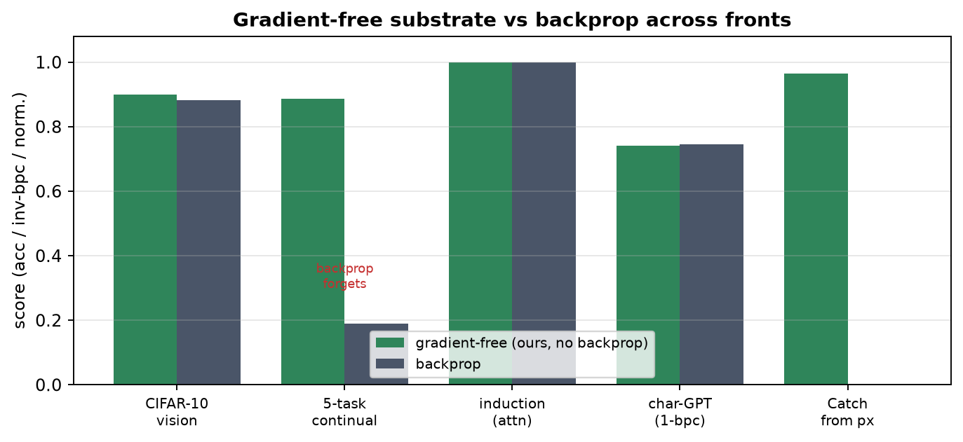
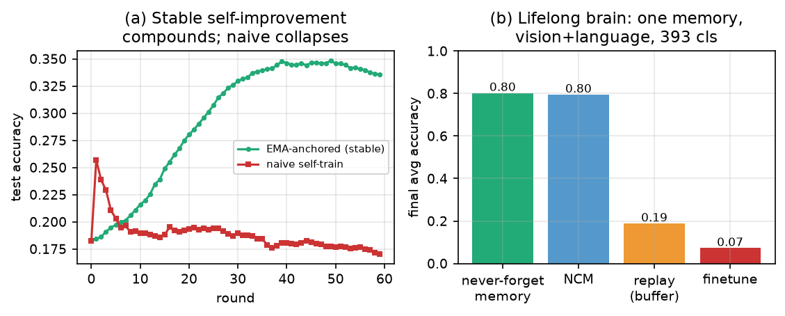
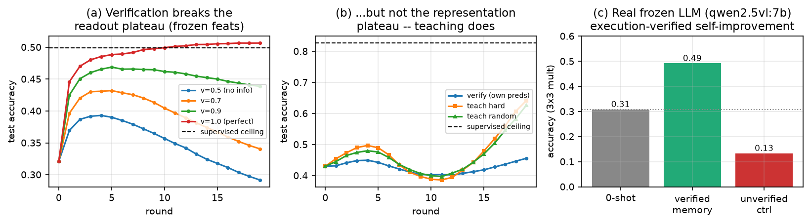
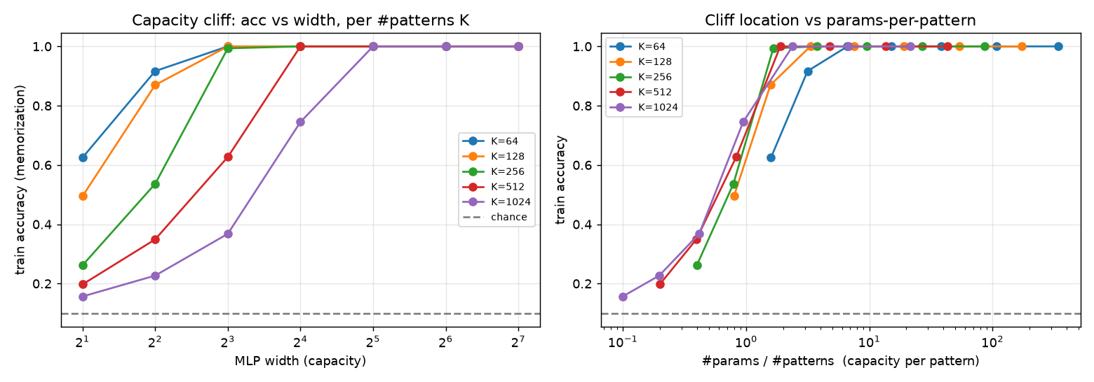
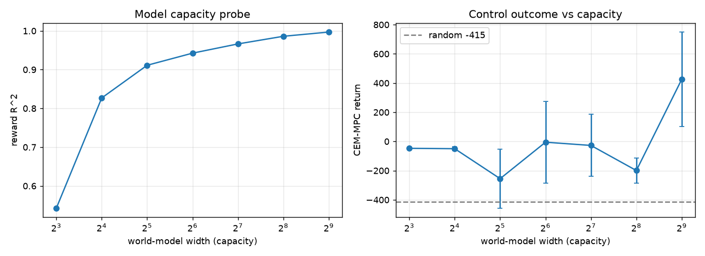
![Fast online adaptation to concept drift. Prequential accuracy on a CIFAR-100/ViT feature stream whose label mapping is re-permuted every $1500$ steps (dotted lines). All three are online update rules on a single linear readout over frozen features (no deep backprop in any). The gated-delta learner (our Gram memory $+$ gate $+$ delta write) recovers fastest after each drift, beating vanilla online accumulation (cannot unlearn) and online SGD on the same readout (adapts too slowly) --- the win is the closed-form error-correcting write, not absence of gradients ([sec:res-online], scoreboard \#112).](assets/results/006-online_drift.png)