Research manuscript · revised scientific draft
Local Evaluation and Continuous Quadratic Forms for Cardinal Spline Networks
Daniel Schmitter
Abstract
Cardinal spline models admit two complementary computational reductions: local evaluation depends on a fixed number of coefficients, while continuous inner products become coefficient-domain quadratic forms. We give a unified formulation of these operations and examine their distinct implementation costs. A cubic layer with 1024 inputs in a batch, 32 input channels, 64 output channels, and 512 coefficients per edge has an archived MPS forward speed ratio of 4.23 and a forward-plus-coefficient-backward ratio of 2.95 for streamed local evaluation relative to dense explicit basis evaluation. Smaller grids favor the dense implementation. The dominant individual intermediates are a 64 MiB dense basis array and an 8 MiB gathered coefficient tap; these are array sizes, not process-memory measurements. Separately, periodic cubic inner products require seven Gram taps, and a circulant inverse action can be computed spectrally. An independent cell-quadrature check agrees with the compact Gram calculation to 2.86 × 10⁻¹⁶ relative error. These results establish a workload-dependent systems opportunity and an exact continuous metric for represented functions, not a universal neural-network speedup or a new spline identity.
1. Introduction
Learnable spline edges combine nonlinear input dependence with a coefficient parameterization that is linear once the input coordinates and basis are fixed. This structure matters for more than approximation. It determines which values must be loaded during evaluation and which continuous losses can be calculated without repeatedly sampling the input domain. KANs make spline edges a visible neural-network component [1], but the underlying local polynomial and inner-product identities are classical [2,3].
We study the interaction between those identities and concrete computational workloads. The contributions are a common derivation of local evaluation and continuous quadratic objectives; a shape-resolved comparison of dense and streamed cubic layers on an archived MPS workload; and a numerical verification of compact and spectral Gram operations. We distinguish algebraic complexity, individual array sizes, observed latency, and differentiation requirements. They do not imply one another.
2. Related work and scope
Local polynomial evaluation, compact support, derivative recurrences, and banded Gram matrices are standard spline properties [2]. Periodic inner-product calculus explicitly relates continuous function geometry to coefficient-domain matrices [3]. Exponential splines extend operator-associated representation beyond polynomials [4]. This paper applies these established facts to operations needed by spline networks; it does not claim to invent matrix evaluation or analytic regularization.
A generic Cox–de Boor evaluator is one comparator for pointwise numerical work, but it is not the only way to implement a KAN. Our neural-layer comparison instead uses an explicit cardinal dense basis, avoiding a false attribution of every improvement to removing recursion. The experiment does not reproduce a complete published KAN training system, measure a custom fused kernel, or compare end-to-end task accuracy.
3. Architecture and information flow
The computational graph has two branches sharing the same trainable coefficients. The prediction branch maps each input to a cell, evaluates its four polynomial weights, gathers the corresponding edge coefficients, and sums over input channels. The regularization branch applies a preassembled operator Gram to the complete coefficient vector. The first branch is data-dependent indexing; the second is a fixed linear map followed by a scalar product. Neither branch requires a generic recursive basis evaluator, but only the second has a data-independent sparsity pattern.
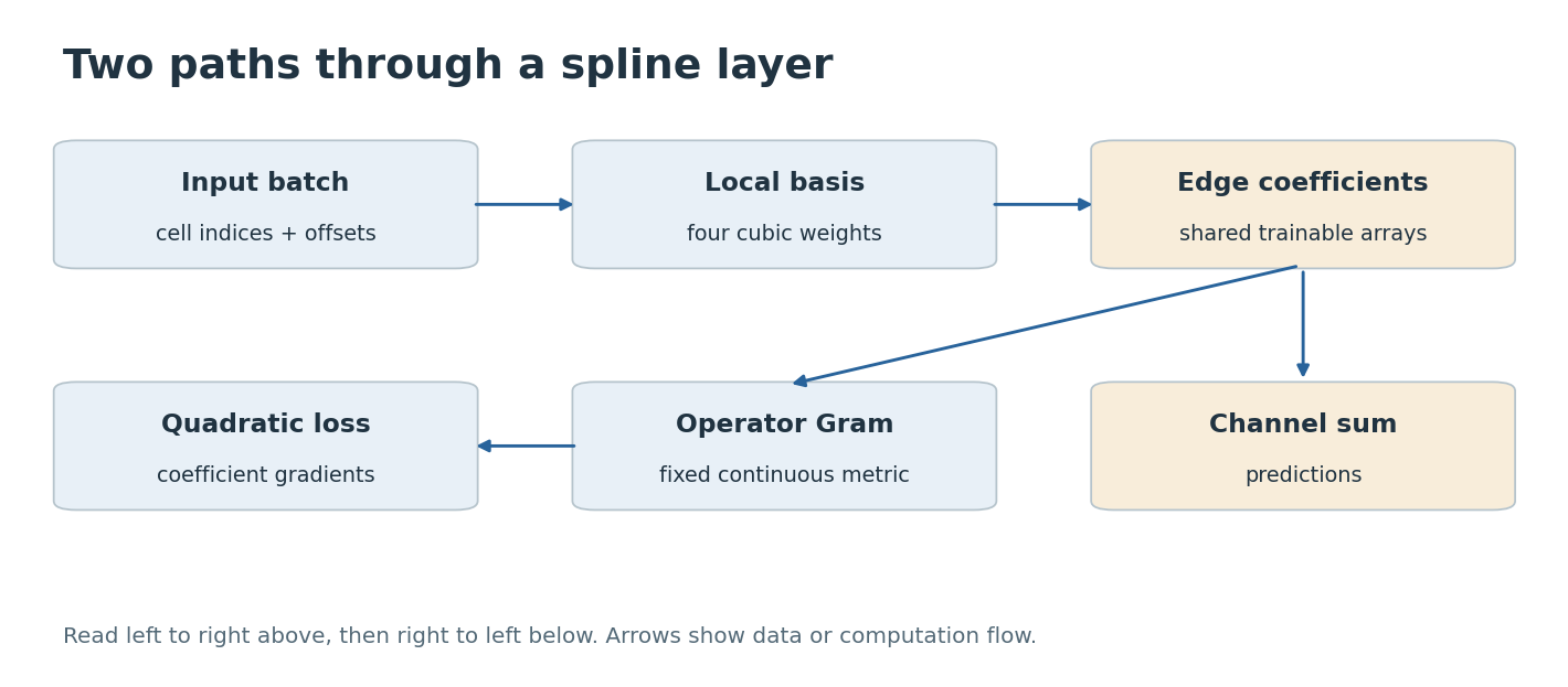
This separation explains why a fast continuous penalty and a fast neural layer are independent claims. The penalty gradient is a structured matrix action. The layer backward pass must additionally accumulate contributions from inputs that address overlapping coefficients. For hidden layers it must propagate derivatives to the input coordinates as well; that path was not timed in the archived coefficient-gradient panel. A local implementation may therefore save an intermediate array while losing to a dense contraction at a small grid.
4. Local cardinal evaluation
Let the knots have spacing h, write x/h=j+t with integer j and , and use centered cubic basis functions. Four coefficients determine the value inside a cell:
Indices are wrapped only for a periodic model. A finite nonperiodic model needs an explicit boundary convention; the layer experiment masks coefficient indices outside its range. The local formula follows by expanding the four cubic pieces on a common cell. Differentiating the monomial row gives the derivative, with a factor of 1/h for each derivative in physical coordinates.
Here B, I, O, and K denote batch size, input channels, output channels, and coefficients per edge. Dense evaluation constructs a B-by-I-by-K basis array and contracts it with I-by-O-by-K coefficients. The local formulation gathers only the four relevant coefficients per edge. Materializing all four taps creates a B-by-I-by-4-by-O array; streaming the taps reduces each individual gather to B-by-I-by-O. Gather traffic, launch overhead, and backward scatter operations can nevertheless make the local route slower than a dense contraction.
The expression is a small matrix-vector product within each cell followed by indexed contractions. It does not automatically become one large tensor-core GEMM: cell indices differ between inputs. Conversely, the dense route may use highly optimized contractions despite evaluating many zero basis entries. These implementation details motivate measuring the crossover instead of inferring speed from operation counts.
5. Continuous objectives and operator structure
For fixed real basis functions and a linear differential operator D with square-integrable basis images, expansion of the integral yields
The matrix is symmetric positive semidefinite. It is positive definite only if the represented space has no nonzero function annihilated by D on the integration domain. Compact support makes entries vanish for nonoverlapping supports. Four-point Gauss integration on each cubic cell exactly integrates products of cubic pieces in real arithmetic; differentiated cubic products require no higher degree. Assembly can therefore be separated from repeated objective and gradient evaluations.
For an unweighted periodic uniform grid, translation invariance further makes the mass matrix G circulant. The autocorrelation of the centered cubic is the centered degree-seven B-spline, giving seven nonzero discrete taps for sufficiently large K:
The first column g determines the real spectral eigenvalues under a consistent discrete-Fourier convention. A seven-tap stencil applies G in linear work; an FFT costs order K log K and need not be faster for that operation. FFT diagonalization is particularly useful for repeated inverse actions. Arbitrary observation locations, spatial weights, variable coefficients, and nonperiodic boundaries generally destroy exact circulant structure. Such problems require their actual matrices, or a justified approximation such as a circulant preconditioner.
A separate operator reduction concerns representation rather than evaluation. If a known linear operator annihilates every basis function, it annihilates their linear combination for any coefficient vector. Measurements then determine coefficients through a linear inverse problem:
For example, sine and cosine modes with a fixed wave number satisfy the corresponding homogeneous Helmholtz equation. This classical null-space construction eliminates a residual penalty only for the encoded equation and space. It does not ensure identifiability, fit arbitrary boundaries, or solve an unknown nonlinear PDE. Exponential-spline reproduction is a wider operator-associated framework [4], but the systems benchmark below evaluates ordinary cubic splines, not exponential kernels.
6. Experimental methods
The point-evaluation panel compares NumPy float64 local cubic evaluation with generic recursion at shapes (B,I,K)=(256,32,16), (512,64,32), and (512,64,64). The separate framework panel fixes B=1024, I=32, O=64 and varies K over 16, 32, 64, 128, 256, and 512. It uses PyTorch float32 on MPS, normally distributed inputs, a finite knot interval from −2.5 to 2.5, and masked out-of-range coefficients. Both routes implement the same layer.
The backward experiment differentiates the mean squared output with respect to coefficients. Input tensors do not require gradients, so it does not measure the input-gradient workload of an internal layer in a deep network. Forward timings retain gradient tracking. The runner uses warm-up calls, device synchronization, and median timings; its default is seven repetitions, but the archived JSON does not retain the actual repetition count, raw repetitions, full hardware identity, or library version. The results are therefore descriptive measurements, not portable performance guarantees or confidence intervals.
The calculus panel uses periodic cubic grids K=64, 256, 1024, and 4096, with batches of 32 coefficient pairs. It compares compact and FFT mass actions and checks a ridge inverse with =0.001. A 32-midpoint-per-cell quadrature is a numerical reference, not an exact integrator. The added bounded consistency test instead uses four Gauss points per cell at K=32 for three random coefficient pairs, with NumPy seed 41802. It reruns no timing or training experiment.
7. Results
| K | Forward ratio | Forward + backward ratio |
|---|---|---|
| 16 | 0.72 | 0.26 |
| 32 | 0.48 | 0.32 |
| 64 | 0.76 | 0.48 |
| 128 | 1.24 | 0.88 |
| 256 | 2.08 | 1.56 |
| 512 | 4.23 | 2.95 |
At K=512, dense and streamed forward latencies are 5.435 ms and 1.286 ms; the corresponding forward-plus-backward latencies are 5.713 ms and 1.937 ms. The maximum absolute output discrepancy for this case is 1.44 × 10⁻⁵ in float32. Small grids favor the dense route, and the backward crossover occurs later than the forward crossover. The archived NumPy recursion comparison gives speed ratios 4.81, 7.09, and 12.19, with discrepancies near float64 roundoff; those are a different CPU workload and must not be reported as GPU neural-layer speedups.
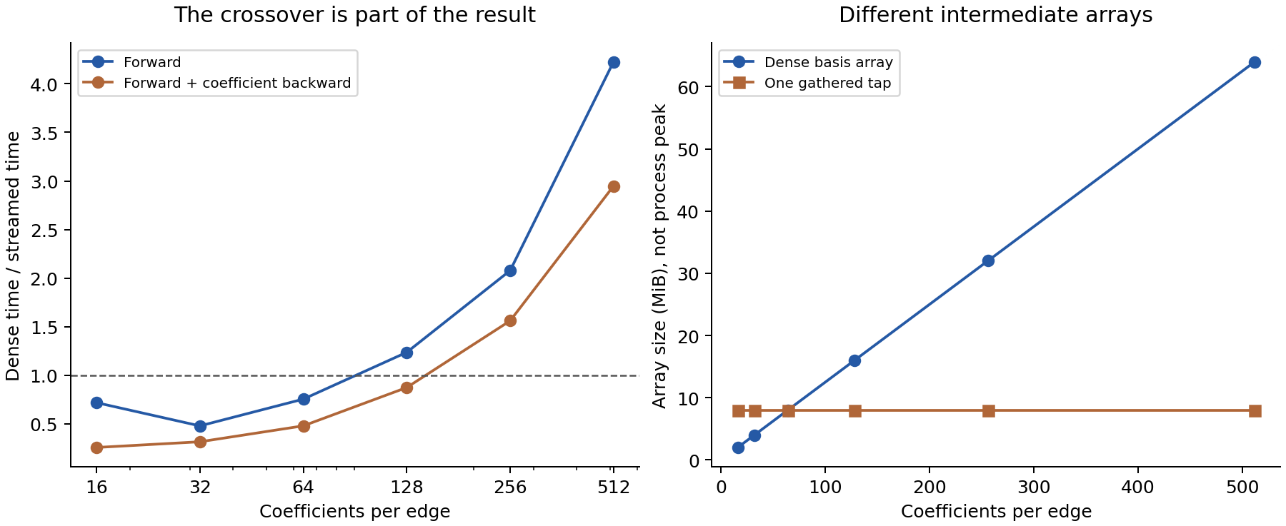
At K=512, the dense basis array occupies 64 MiB, compared with 8 MiB for one gathered tap and 32 MiB for a materialized four-tap gather. Multiple arrays, coefficients, outputs, and autograd state remain live; the 8 MiB quantity is not a total-memory claim. At K=4096, a dense float64 Gram matrix would occupy 128 MiB, whereas the stored kernel and spectrum occupy approximately 0.0625 MiB. A compact seven-tap implementation is also a necessary and much smaller comparator than a dense matrix.
Compact and FFT Gram actions agree to at most 1.09 × 10⁻¹⁵ relative error, and the ridge inverse residual is at most 1.03 × 10⁻¹⁵. Midpoint integration differs by up to 2.67 × 10⁻⁸, reflecting its discretization. The independent four-point cell check reduces the relative discrepancy to 2.86 × 10⁻¹⁶. This verifies continuous mass calculus; it is not a measured tenfold speedup of a neural-network inner-product loss.
8. Discussion and reproducibility
Cardinal structure removes a dependence on K from the number of active coefficients at an input, but hardware execution still determines latency. Continuous quadratic forms remove repeated numerical integration only when the basis, operator, weight, and domain permit reusable assembly. Learned moving coordinates or basis parameters can require rebuilding or differentiating that assembly. These constraints identify useful workloads more precisely than a universal claim that matrix multiplication solves spline efficiency.
The supplement contains the complete source measurement records, hashes, and independent consistency result. Source runners and their dependency notes accompany the paper. The legacy calculus runner contains unnecessarily large temporary allocations in its high-resolution quadrature path; the independent check deliberately avoids that path. No historical benchmark was rerun for this manuscript. End-to-end optimization, fused-kernel performance, input gradients, peak memory, energy, and edge-device deployment remain unmeasured.
9. Application boundary and research implication
A useful integration would place these operations behind one layer interface with separate preparation, forward, input-gradient, and coefficient-gradient measurements. The existing evidence qualifies local large-grid evaluation and continuous mass arithmetic, not an entire training system. The architecture identifies exactly which additional measurements would be needed before claiming lower training cost.
10. Conclusion
Local cell evaluation and continuous coefficient geometry provide complementary tools for spline networks. The first has a measured large-grid advantage and small-grid disadvantage on the reported MPS layer; the second exactly represents declared continuous quadratic objectives and supports structured linear algebra. The practical contribution is to make those mechanisms and their limits explicit enough to select and verify an implementation, without conflating them with an accuracy or universal training-speed claim.
References
- Z. Liu et al. KAN: Kolmogorov–Arnold Networks. arXiv:2404.19756, 2024. Source
- C. de Boor. A Practical Guide to Splines. Revised edition. Springer, 2001. Source
- A. Badoual, D. Schmitter, and M. Unser. An Inner-Product Calculus for Periodic Functions and Curves. IEEE Signal Processing Letters, 23(6), 878–882, 2016. Source
- M. Unser and T. Blu. Cardinal Exponential Splines: Part I—Theory and Filtering Algorithms. IEEE Transactions on Signal Processing, 53(4), 1425–1438, 2005. Source