Research manuscript · revised scientific draft

Function-Preserving Grid Transfer and Continuous Regularization in Spline Networks

Daniel Schmitter

Abstract

Increasing the resolution of a spline network changes its parameterization and can perturb its predictions before any new learning occurs. We study this transition in periodic cubic spline edges using continuous cross-Gram projection, and separate the effects of parameter transport, additional capacity, and curvature regularization. Projection preserves the represented function under nested refinement and minimizes continuous squared error for nonnested transfer or restriction. These are classical spline-space properties; our contribution is their explicit integration and controlled evaluation as a network-growth primitive. A six-edge additive network refined from 24 to 96 coefficients per edge exhibits median relative function drift of 1.97 × 10⁻¹⁵, compared with 2.63% for coefficient interpolation. On five independently seeded noisy high-frequency regression problems, a fixed curvature penalty reduces median test mean-squared error from 2.2615 × 10⁻⁵ to 2.0896 × 10⁻⁵ after refinement. The competing warm starts attain almost identical final errors, and an already-resolved smooth problem deteriorates after growth. Thus exact transport removes a parameterization artifact; it does not by itself establish better generalization. An independent consistency test confirms agreement with classical dyadic refinement and full-rank sampled least-squares transfer.

1. Introduction

Learnable univariate functions provide a natural mechanism for increasing the resolution of a neural network without changing its connectivity. Kolmogorov–Arnold networks (KANs) make this possibility explicit through spline grid extension [1]. The transition is nevertheless a numerical operation: a function represented on one grid must be represented on another. A change in prediction caused by this operation is distinct from a change caused by training.

This distinction matters when a trained component is enlarged during continued optimization, particularly when its output is consumed immediately by another model. It also matters experimentally. If a refinement method changes the inherited function, a comparison of subsequent learning curves confounds initialization quality with additional representational capacity. Function-preserving transformations have a broader precedent in Net2Net [2]; spline spaces supply their own classical refinement and projection operators [3,4].

We investigate a continuous-space transfer operator for periodic cubic spline edges, together with a curvature penalty evaluated in coefficient space. The study makes three contributions: a self-contained formulation of the invariants needed at a grid transition; a comparison that isolates transition error from post-transition learning; and a paired assessment of exact continuous regularization on an unresolved target. We also report an already-resolved target for which growth is detrimental. The scope is a small additive network, not a new universal network architecture or a general KAN-versus-MLP benchmark.

2. Related work

B-spline refinement, knot insertion, orthogonal projection, and derivative penalties predate neural spline models [3,4]. Badoual, Schmitter, and Unser formulate inner products of periodic functions through coefficient-domain matrices [3]. We use this calculus to express both inter-grid projection and curvature energy. We do not claim these identities or the existence of exact nested refinement as new mathematical results.

The original KAN grid-extension procedure refits a finer spline to values of the coarse spline using least squares [1, Sec. 2.4]. For nested spaces and a full-column-rank evaluation matrix, sampled least squares can also recover the function exactly. Continuous projection therefore is not contrasted with an intrinsically inexact KAN procedure. Its distinctive specification is the continuous-domain approximation criterion, independent of a chosen activation sample distribution, and its applicability to nonnested transfer and coarsening. Coefficient interpolation and assigning knot values directly to coefficients are diagnostic controls, not faithful reproductions of the original KAN refit.

Net2Net develops function-preserving enlargement for conventional neural networks [2]. Here the connectivity is fixed and the internal degrees of freedom of an edge increase. Classical smoothing splines penalize integrated derivatives [4]. Our curvature term uses that same principle after network refinement. The experimental contribution is the separation of these mechanisms and their observed effects, rather than a claim that function preservation or smoothness regularization is unprecedented.

3. Network architecture and learning interface

The tested network has six scalar inputs, six trainable univariate edge functions, and one summation output. There are no hidden layers or learned input-coordinate transforms. Each edge expands a fixed periodic cubic basis. The training observations are six-dimensional input vectors and noisy scalar labels; individual target-edge values are not supplied as supervision. This distinction makes the aggregate fitting task different from independently fitting six labeled curves.

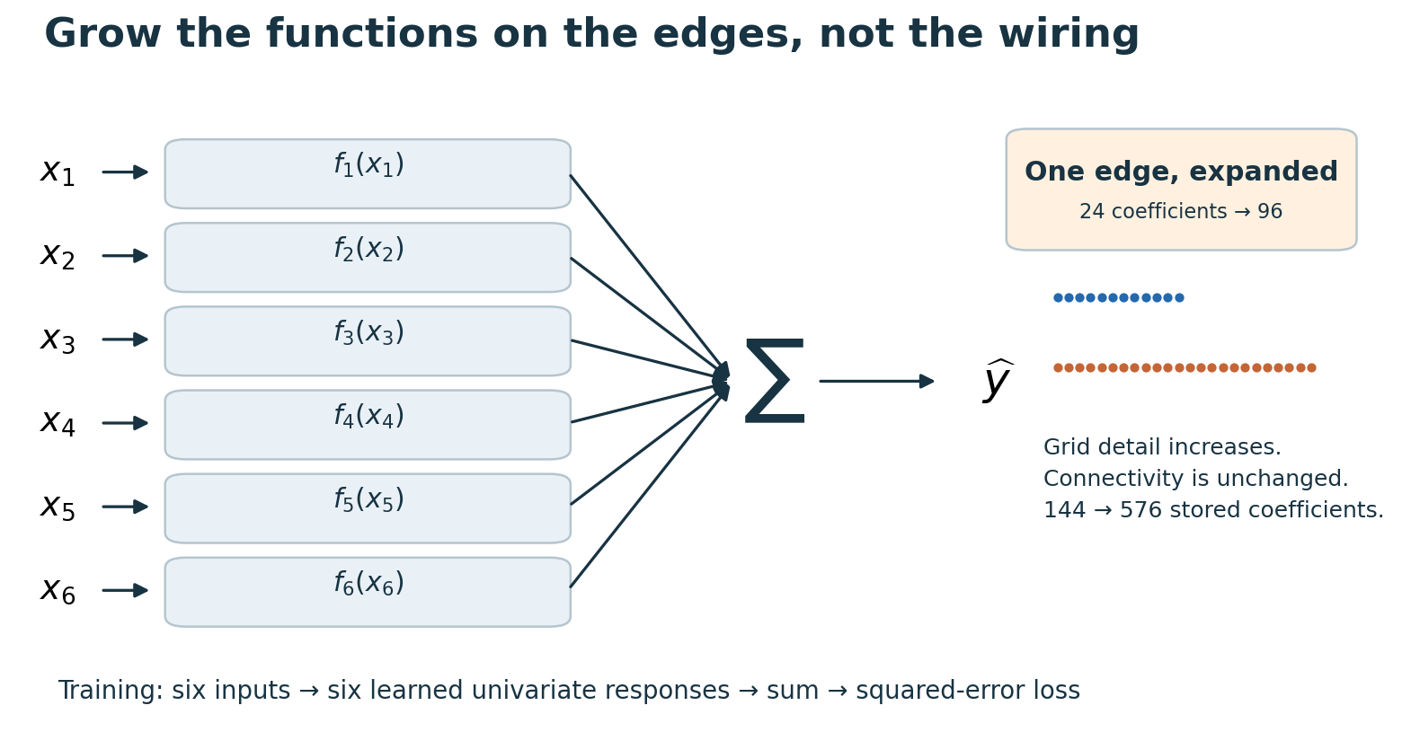
Actual additive-network architecture. Each input passes through its own learned spline response before summation. Growth changes each edge from 24 to 96 coefficients, leaving all six input connections and the output operation fixed. Dots in the inset schematically indicate a finer grid, not one dot per coefficient.

x\in[0,1]^6\longmapsto z(x)=\big[\phi_m(x_1);\ldots;\phi_m(x_6)\big],\qquad \widehat y=z(x)^Tc,\quad c\in\mathbb R^{6m}.

The coarse model stores 144 coefficients and the fine model stores 576. Since every edge can represent a constant, moving a constant between two edges leaves their sum unchanged. Five such gauge directions make individual edge offsets unidentifiable from aggregate labels. The corresponding additive function-space dimensions are 139 and 571, respectively. Exact transport preserves the chosen coefficient representation edge by edge, while predictive evaluation concerns their sum.

The archived controlled sequence. A single coarse checkpoint feeds every transfer arm. New Adam optimizers are created after transfer, so optimizer-moment preservation is not being tested. Immediate drift and post-training error answer distinct questions.

4. Periodic spline spaces and transfer

Let $\beta_3$ be the centered cubic B-spline with support [−2,2]. On the unit circle, define the periodized basis and its span by

\phi_{m,j}(x)=\sum_{\ell\in\mathbb Z}\beta_3(mx-j-\ell m),\quad j=0,\ldots,m-1,\qquad V_m=\operatorname{span}\{\phi_{m,j}\}_{j=0}^{m-1}.

All inner products below are unweighted integrals over [0,1]. For source coefficients c and target coefficients d, write $f=\Phi_m c$ and $g=\Phi_n d$ . The implementation uses $m,n\ge8$ , for which nearest-period evaluation agrees with the periodized compact support. The basis is linearly independent, and its functions form a partition of unity.

(A_n)_{ij}=\langle\phi_{n,i},\phi_{n,j}\rangle,\qquad (C_{n,m})_{ij}=\langle\phi_{n,i},\phi_{m,j}\rangle,\qquad d=P_{n,m}c=A_n^{-1}C_{n,m}c.

The matrix $A_n$ is symmetric positive definite. Expanding the squared approximation error gives a quadratic form in d. Its unique stationary point is the displayed transfer, and its positive-definite Hessian makes that point the unique minimizer.

\|\Phi_n d-\Phi_m c\|_{L^2}^2=d^TA_nd-2d^TC_{n,m}c+c^TA_mc.

Proposition 1 (projection consequences). The transferred function is the $L^2$ -orthogonal projection of f onto $V_n$ . Consequently (i) it preserves f whenever $V_m\subseteq V_n$ ; (ii) it preserves the integral of f; and (iii) its error is no greater than that of any other function in $V_n$ . These statements concern functions, not equality of their coefficient arrays.

Proof. The normal equation gives $\langle g-f,v\rangle=0$ for every $v\in V_n$ . If $f\in V_n$ , choose $v=g-f$ to obtain $g=f$ . Since $1\in V_n$ , choosing $v=1$ proves equality of integrals. For any h∈ $V_n$ , orthogonality yields $\|f-h\|^2=\|f-g\|^2+\|g-h\|^2$ , proving optimality. These are standard orthogonal-projection arguments applied to the present spline spaces.

Integer refinement $n=qm$ is nested for a common periodic domain and aligned knot origin. Nonnested grids, translated grids, a changed domain, or changed boundary conventions do not inherit exact preservation merely because n exceeds m. Under nested refinement, transferring back to the coarse space also recovers the original function and coefficients in exact arithmetic.

For a sum of unchanged edge functions, exact edge transfer preserves the network output at every input, not merely at training samples. The same argument extends layer by layer to a composition if every edge is preserved over its entire relevant domain and the other operations and input coordinates are unchanged. It does not describe the subsequent optimizer trajectory.

5. From edge projection to network error

Projection preserves each edge integral. This gives an additional network-level interpretation when inputs are independent and uniform on the declared domain. Let each edge residual be the transferred function minus its original. Every such residual then has zero mean. Expanding the squared sum and integrating over the product domain eliminates the cross terms:

\int_{[0,1]^E}\left(\sum_e r_e(x_e)\right)^2dx=\sum_e\int_0^1r_e(x)^2dx,\qquad \int_0^1r_e(x)dx=0.

Thus the continuous edge errors add exactly at the additive-network output under this product measure, even for nonnested projection. This is a consequence of orthogonality, not a general guarantee for correlated activations or deep compositions. A new bounded six-edge 24-to-36 projection check gives both sides as 0.0005507010128079836, with maximum absolute edge-error mean 4.22 × 10⁻¹⁷. The check uses seed 7500 and exact cell quadrature; it performs no learning and does not replace the archived task evaluation.

6. Assembly, refinement, and regularization

We assemble $A_n$ and $C_{n,m}$ on the union of the source and target knot partitions. On each interval their integrands are polynomials of degree at most six. Four-point Gauss–Legendre quadrature integrates such polynomials exactly in real arithmetic. The code performs dense assembly and a dense solve, using one right-hand side per edge. Exact integration does not imply exact floating-point arithmetic.

Because $A_n$ is circulant on the uniform periodic grid, its inverse action can alternatively be diagonalized by the discrete Fourier transform. The archived transfer timings use the dense solve and exclude assembly; they are not evidence of an FFT speedup. The cross-grid matrix is rectangular and cannot generally be replaced by an arbitrary single-grid circulant filter.

For dyadic refinement, the classical two-scale mask provides an especially simple independent implementation:

\beta_3(t)=\sum_{k=-2}^{2}h_k\beta_3(2t-k),\qquad (h_{-2},h_{-1},h_0,h_1,h_2)=\tfrac18(1,4,6,4,1),\qquad d_{(2j+k)\bmod 2m}\mathrel{+}=h_kc_j.

This local operation has linear work in the number of coefficients and is preferable to a dense projection solve when dyadic nested refinement is the only operation needed. Projection provides a common formulation that also covers restriction and nonnested grids. The independent consistency check compares both implementations, rather than presenting projection as a superior replacement for classical refinement.

The continuous curvature penalty for an edge is an exact quadratic form. For E edges, the objective used after refinement is

R_{n,ij}=\int_0^1\phi''_{n,i}(x)\phi''_{n,j}(x)\,dx,\qquad \mathcal J(d)=\frac1N\sum_{i=1}^{N}\big(\widehat y_d(x_i)-y_i\big)^2+\frac\lambda E\sum_{e=1}^{E}d_e^TR_nd_e.

Second derivatives of cubic pieces are linear, so two-point Gauss integration per cell already suffices; the implementation reuses the four-point rule. $R_n$ is positive semidefinite and includes the physical $n^2$ derivative scaling on the unit domain. For an exact embedding matrix P, $P^T R_n P=R_m$ : the same function has the same curvature energy on either grid. Thus $\lambda$ retains a function-space meaning under refinement, unlike an unscaled coefficient-difference penalty.

Prescribed linear boundary data can be incorporated in a different, nonperiodic model by writing $c=c_0+Nz$ , with $Bc_0=b$ and $BN=0$ . This familiar null-space parameterization fixes the boundary conditions while optimizing z. It is not part of the periodic experiments reported here; a transfer into such a space requires the corresponding constrained projection.

7. Experimental methods

The transfer-only panel contains six grid pairs: 24→48, 24→96, 48→72, 64→32, 64→24, and 64→16. Each pair uses 32 random coefficient vectors combining sinusoidal, localized Gaussian, and Gaussian-noise terms, generated sequentially from NumPy seed 20260911. Continuous errors are integrated on the union partition. A separate random-coefficient 24→96→24 test measures round-trip coefficient error. The panel is a numerical mechanism check, not 192 independent application tasks.

The learning panel uses the additive predictor $\widehat y(x)=\sum_e f_e(x_e)$ , with six periodic cubic edges. Each seed generates 4096 independent training inputs and 4096 test inputs uniformly on $[0,1]^6$ . The target is a sum of scalar edge responses:

\begin{aligned}f_e^\star(x)={}&(0.55+0.04e)\sin(2\pi x+0.37e)+0.20\cos(6\pi x-0.185e)\\&+0.16\exp\!\left[-\left(\frac{\delta(x,\mu_e)}{0.035}\right)^2\right]+0.08\sin(30\pi x+0.23e).\end{aligned}

\mu_e=(0.13+0.117e)\bmod1,\quad e=0,\ldots,5.

Here $e=0,\ldots,5$ and $\delta$ is the signed shortest periodic displacement. Independent Gaussian noise with standard deviation 1% of the clean training-target standard deviation is added to training labels; test labels are clean. The wrapped Gaussian is evaluated as specified even though its derivatives at the antipode are not analytically periodic; the resulting discontinuity in those derivatives is exponentially small at the stated width.

Each 24-coefficient edge starts at zero. Full-batch Adam runs for 500 steps with learning rate 0.03. The same coarse checkpoint initializes four 96-coefficient arms: continuous projection, periodic linear interpolation of coefficient arrays, source values at target knots assigned as coefficients, and zero restart. Every arm receives a fresh Adam optimizer and 250 further steps with learning rate 0.015. The implementation uses float64. Immediate drift is evaluated on 8192 uniformly spaced points per edge; learning-curve errors are logged every ten steps. A reported recovery step is therefore a logged checkpoint, not necessarily the first update that recovered.

The regularization parameter $\lambda$ =10⁻⁹ was selected on earlier development runs and held fixed for the paired five-seed panel with seeds 20260920 through 20260924. These integers are random seeds, not dates of execution. The unregularized and regularized runs use identical generated observations and initial checkpoints. The test set is evaluated repeatedly to record curves, but the reported endpoint is the fixed 250-step endpoint, not the best observed test checkpoint. With five seeds, paired improvements are descriptive evidence for this task family, not a precise population-level effect estimate.

8. Results

Continuous transfer errors. Medians over 32 coefficient vectors per row; dimensionless relative L² error.
Source → target	Projection	Coefficient interpolation	Values as coefficients
24 → 48	9.43 × 10⁻¹⁶	1.71 × 10⁻²	9.52 × 10⁻³
24 → 96	1.62 × 10⁻¹⁵	2.30 × 10⁻²	2.51 × 10⁻³
48 → 72	6.00 × 10⁻⁴	5.28 × 10⁻³	7.74 × 10⁻³
64 → 32	1.94 × 10⁻²	4.35 × 10⁻²	3.50 × 10⁻²
64 → 24	2.58 × 10⁻²	5.18 × 10⁻²	5.02 × 10⁻²
64 → 16	3.28 × 10⁻²	8.47 × 10⁻²	8.48 × 10⁻²

Nested projection has worst relative $L^2$ error 1.71 × 10⁻¹⁵. The round-trip coefficient error is 1.18 × 10⁻¹⁵. Projection preserves the integral to at most 1.39 × 10⁻¹⁶ across the six transfer cases. Nonnested refinement and coarsening have nonzero approximation error, as expected, but projection improves the median over both diagnostic controls in each case.

Noisy high-frequency learning panel. Medians over the same five seeds, λ=10⁻⁹. Drift and loss ratio are measured immediately after transfer; final MSE is measured after 250 updates.
Initialization	Relative drift	Loss ratio	Final test MSE
Continuous projection	1.97 × 10⁻¹⁵	1.0000	2.08964 × 10⁻⁵
Coefficient interpolation	2.63 × 10⁻²	1.0567	2.08963 × 10⁻⁵
Values as coefficients	2.63 × 10⁻³	0.9989	2.08964 × 10⁻⁵
Zero restart	1.0000	70.9825	2.13098 × 10⁻⁵

Exact transport removes the instantaneous prediction change. It does not produce a meaningful final-error advantage over the other nonzero warm starts on this task: their final medians differ by less than four parts per million. The values-as-coefficients control even slightly reduces the immediate loss on the median case despite perturbing the function. Function invariance and lower task loss are different properties.

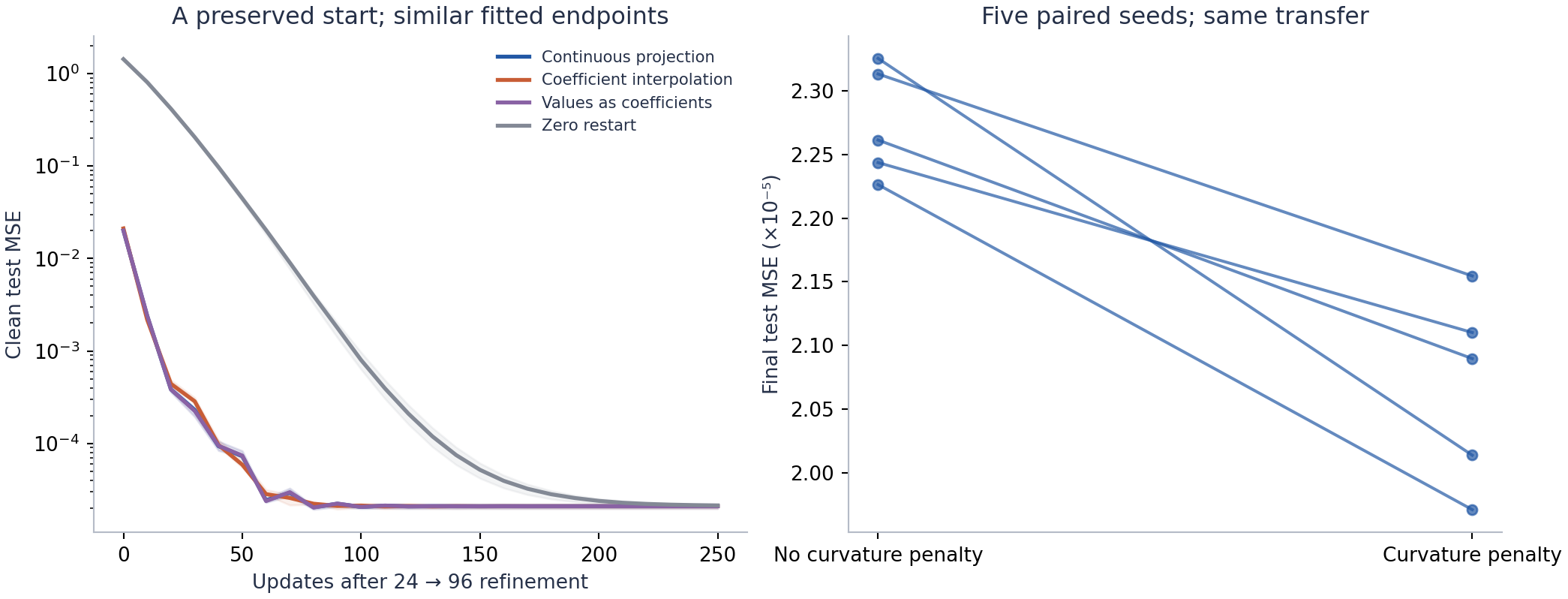
Archived learning trajectories and paired regularization outcomes. Left: median clean test MSE across five seeds, with shaded minimum-to-maximum ranges, not confidence intervals. Curves begin after refinement; the unchanged coarse model has median MSE 0.020122. Right: each segment joins the same seed without and with λ=10⁻⁹. All plotted values come from the stored experiment JSON, not an illustrative animation.

For exact transfer, curvature regularization lowers the median final MSE from 2.26150 × 10⁻⁵ to 2.08964 × 10⁻⁵. It improves all five paired seeds, with geometric mean unregularized-to-regularized error ratio 1.100. The large reduction relative to the 24-knot checkpoint, whose median MSE is 0.020122, primarily reflects resolution of a deliberately unresolved target. It must not be attributed entirely to the transfer operator or to the comparatively small regularization effect.

A historical smooth-target panel exhibits the opposite capacity effect: the coarse model has median MSE 5.02 × 10⁻⁶, whereas unregularized exact refinement reaches 2.24 × 10⁻⁵ after training. The immediate transfer still preserves the function. This is a counterexample to the implication that a preserved transition guarantees a beneficial enlargement. The stored configuration for this earlier panel omits the target-detail fields added to the current runner. We therefore report it as a historical diagnostic rather than claiming it is fully reproduced by the current defaults.

9. Independent consistency checks and reproducibility

An additional numerical check compares continuous projection with the explicit dyadic mask for $m\in\{8,24,48\}$ . For each size it also solves a sampled least-squares transfer on 4m uniformly spaced, offset samples. Four random coefficient vectors are tested at 997 independently generated off-grid locations, using seed 41018. Relative discrepancies of projection versus mask, off-grid function values, sampled-refit coefficients, and normal-equation residuals are each required to be below 10⁻¹². All twelve size-by-check comparisons pass. This is a consistency test of classical identities, not a newly held-out generalization experiment.

The supplementary files include the exact JSON results, experiment configuration, plotting code, and SHA-256 source fingerprints used for the figures. The original transfer and training runners are retained unchanged. The added script performs only arithmetic verification and figure extraction; it does not retrain the networks or choose a new regularization coefficient. Training timings are not used to claim a hardware advantage.

10. Discussion and limitations

The principal practical result is a clean separation between representation changes and learning changes. An exact transition can preserve outputs and continuous regularizers while exposing additional degrees of freedom. Whether those degrees of freedom are useful remains a statistical question. A subsequent validation-based growth decision is a reasonable design implication, but an automated selector with an untouched final evaluation is not tested here.

The additive network is linear in its coefficients despite being nonlinear in its input coordinates. A regularized least-squares solve is therefore a natural alternative to Adam and a necessary comparator for an optimization-efficiency claim. We used Adam to study a checkpoint transition under a fixed continued-training protocol; the experiment does not establish that iterative optimization is necessary or optimal. Nor does it test deep KANs with changing hidden coordinates, nonperiodic tails, adaptive knot relocation, or transport of Adam moments.

Exact sampled refitting and classical refinement are strong baselines for nested enlargement, as the independent checks confirm. The heuristic controls reveal the consequences of incorrect parameter transport, not a universal defect in existing KAN software. The continuous-space formulation becomes most distinctive when the desired criterion is an integral over a declared domain or when the new space is not nested. Comparisons on activation-weighted versus uniform-domain risk may favor different projections.

11. Conclusion

Continuous spline calculus supplies a well-defined network-growth primitive: preserve the represented function when the spaces are nested, otherwise compute its best $L^2$ approximation, and evaluate smoothness in the same continuous metric. The experiments verify the transition invariants and a modest paired regularization benefit on an unresolved synthetic task. They also show near-equal fitted endpoints for several warm starts and deterioration on an already-resolved target. These findings support using exact transfer to remove an avoidable numerical perturbation, while keeping decisions about capacity and generalization separate.

References

Z. Liu, Y. Wang, S. Vaidya, F. Ruehle, J. Halverson, M. Soljačić, T. Y. Hou, and M. Tegmark. KAN: Kolmogorov–Arnold Networks. arXiv:2404.19756, 2024; version 5, 2025. Source
T. Chen, I. Goodfellow, and J. Shlens. Net2Net: Accelerating Learning via Knowledge Transfer. ICLR, 2016. Source
A. Badoual, D. Schmitter, and M. Unser. An Inner-Product Calculus for Periodic Functions and Curves. IEEE Signal Processing Letters, 23(6), 878–882, 2016. Source
C. de Boor. A Practical Guide to Splines. Revised edition. Springer, 2001. Source