Research manuscript · revised scientific draft
Learning Constitutive Laws Inside Known Dynamics: Structured Identification and Out-of-Range Prediction
Daniel Schmitter
Abstract
Learning a dynamical vector field and learning an unknown constitutive relation allocate statistical capacity differently. We examine that distinction for one-dimensional viscous conservation laws with known diffusion and transport structure. Fixed linear-in-coefficient constitutive models are fitted to short trajectories and inserted into the same numerical solver for longer, higher-amplitude prediction. Across three archived seeds, a sparse polynomial–trigonometric dictionary gives median normalized extrapolation error 9.29 × 10⁻⁷ for an oscillatory flux contained in its candidate span, compared with 0.0648 for a degree-five polynomial flux, 0.330 for a direct cardinal KAN residual, and 0.298 for a direct MLP residual. On a saturating flux outside the finite dictionary, its median error is 0.00520. Local spline tails perform substantially worse under amplitude shift. A separate noisy flux–reaction experiment supports weak-form fitting at 1% noise, but a weak polynomial control outperforms the sparse dictionary at 2% noise. The results support structural placement of learning and appropriate extrapolating libraries, not a universal KAN ranking or exact discovery of arbitrary physics.
1. Introduction
A model of a physical process often contains both established equations and an unknown response law. Treating the entire right-hand side as an unconstrained regression problem asks data to recover structure that is already available. Conversely, a restrictive constitutive library can make extrapolation appear easy when it contains the generating law. Both effects must be visible in an evaluation.
We study a controlled family in which conservation, viscosity, and the numerical evolution method are known, while the scalar flux is learned. Our contribution is an explicit comparison between local constitutive splines, global polynomial–trigonometric libraries, polynomial controls, and direct neural residual models, together with a noisy weak-form extension. All reported learning runs are archived experiments. The manuscript reorganizes and analyzes those results without additional tuning or training.
2. Related work
Sparse identification of nonlinear dynamics uses a candidate library to identify compact governing equations [1]. The polynomial control here is ridge regression, not a faithful implementation of every sparsity mechanism in SINDy. Weak-form identification transfers derivatives onto test functions to reduce sensitivity to observation noise [2]. We use that established principle and do not claim integration by parts as a new discovery.
KANs parameterize neural edges by univariate functions [3]. Their inclusion here asks whether a direct learned residual is competitive with learning only a constitutive component. It is not an architecture-only comparison: the structured models receive additional factorization information. Operator-associated exponential splines reproduce exponential-polynomial components [4]. Our finite trigonometric dictionary is inspired by this operator view but is not an exponential B-spline implementation. A favorable dictionary result must not be renamed a demonstrated spline-specific advantage.
3. Architecture and information flow
The structured learner has a single trainable physical interface: a scalar constitutive flux. Measured trajectories produce a regression system; its fitted coefficients define the flux; the same numerical evolution operator then produces test trajectories. In the noisy extension, flux and reaction each receive their own dictionary columns. The direct KAN and MLP controls instead learn the non-diffusive state derivative from state and gradient. Their output enters the solver at a different location. The diagram therefore displays an architectural comparison, not interchangeable networks with identical prior information.
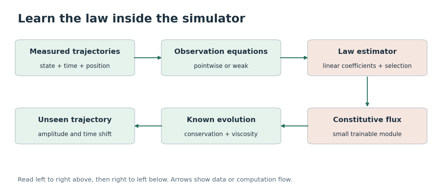
Two sources of extrapolation must be distinguished. Conservation supplies the assembly rule that turns a flux into a state derivative. The global library supplies behavior outside the visited state range. The first does not determine the second: an accurately fitted local spline can still have an unsuitable continuation beyond its supported amplitudes. Likewise, the additive constant in a flux is invisible to its spatial derivative, so identifying the physical evolution does not identify every coefficient convention.
4. Problem formulation
The spatial domain is periodic. Once the scalar basis is fixed, identifying the flux is linear in its coefficients even though evolution is nonlinear in the state. Pointwise observations give a regression design through the chain rule:
Adding a constant to the flux leaves the equation unchanged. The polynomial and trigonometric libraries omit an independent constant term; flux-error comparisons remove the mean difference. The observation matrix must still contain enough excitation to identify its active columns. A small residual on an unvisited state range conveys no information about the flux there.
Three generating laws separate an exactly polynomial case, a dictionary-matched oscillatory case, and a nonpolynomial case outside the finite dictionary:
The global dictionary contains u, u squared, u cubed, and sine/cosine pairs at integer frequencies one through six: fifteen candidates. Columns are RMS-scaled. The selection procedure examines singletons and pairs and then greedily adds terms, with up to six active terms, using the training Bayesian information criterion. This is discrete candidate selection, not continuous learning of arbitrary poles. Correlated space–time rows limit a literal independent-sample interpretation of that criterion.
Other structured controls are a 25-center local cubic spline on the declared state range [−1.35,1.35], a degree-five polynomial, a linear residual, a cubic-polynomial-plus-local residual, and an atlas-plus-local residual. Local residual fitting uses ridge coefficient 0.0001. The main global fits use a trace-scaled ridge of 10⁻⁸. The word atlas denotes the finite dictionary above, not a learned collection of unrestricted charts.
5. Experimental methods
Each of three seeds, 20260910 through 20260912, generates six training trajectories on 64 spatial points. Initial conditions combine three randomized harmonics, normalized to amplitude budget 0.65, and a uniform offset between −0.08 and 0.08. RK4 uses time step 0.002 for 100 steps. Centered time differences at stride four yield 25 snapshots per trajectory and 9600 regression rows. Spatial derivatives are spectral. These rows are dependent observations within six trajectories, not 9600 independent replications.
Evaluation uses 400 steps, an amplitude budget of 1.05 for amplitude-shift cases, and 128 spatial points for resolution-shift cases. Four separately generated initial-condition cases cover in-distribution, amplitude, resolution, and joint shifts for each law and seed. Because initial conditions differ between modes, the resolution comparison is not a paired mesh-convergence test. The principal outcome reported here is amplitude-shift rollout error over steps 101–400, beyond the training time horizon, normalized by the reference trajectory standard deviation in that window.
Reference and structured models share RK4, viscosity, and a spectral flux derivative after a two-thirds-frequency cutoff. The pointwise regression uses the continuous chain rule, whereas the solver differentiates a discretized, filtered flux. Their finite-grid mismatch need not be zero even when the exact law is representable. Rollout accuracy, rather than a training residual alone, tests the resulting model.
The direct residual controls take state and spatial gradient as inputs, learn the non-diffusive right-hand side, and retain the same known viscous term. The in-house cardinal KAN has widths 2–8–1, thirteen knots, a SiLU base path, and 345 parameters. The tanh MLP has widths 2–16–16–1 and 337 parameters. Both use normalized inputs and targets, float32 Adam with learning rate 0.002, 1200 updates, and batches of 4096 rows. The structured regressions use float64. Neither architecture search nor equal-compute optimization was performed; the comparison is between these specified methods, not their best attainable variants.
6. Results
| Model | Oscillatory flux | Saturating flux |
|---|---|---|
| Local cubic spline | 0.1870 | 0.1644 |
| Polynomial + local | 0.1423 | 0.0778 |
| Sparse global atlas | 9.29 × 10⁻⁷ | 0.00520 |
| Atlas + local | 4.27 × 10⁻⁵ | 0.00519 |
| Polynomial degree 5 | 0.0648 | 0.0411 |
| Linear residual | 0.4538 | 0.3332 |
| Direct cardinal KAN | 0.3300 | 0.1839 |
| Direct MLP | 0.2977 | 0.1165 |
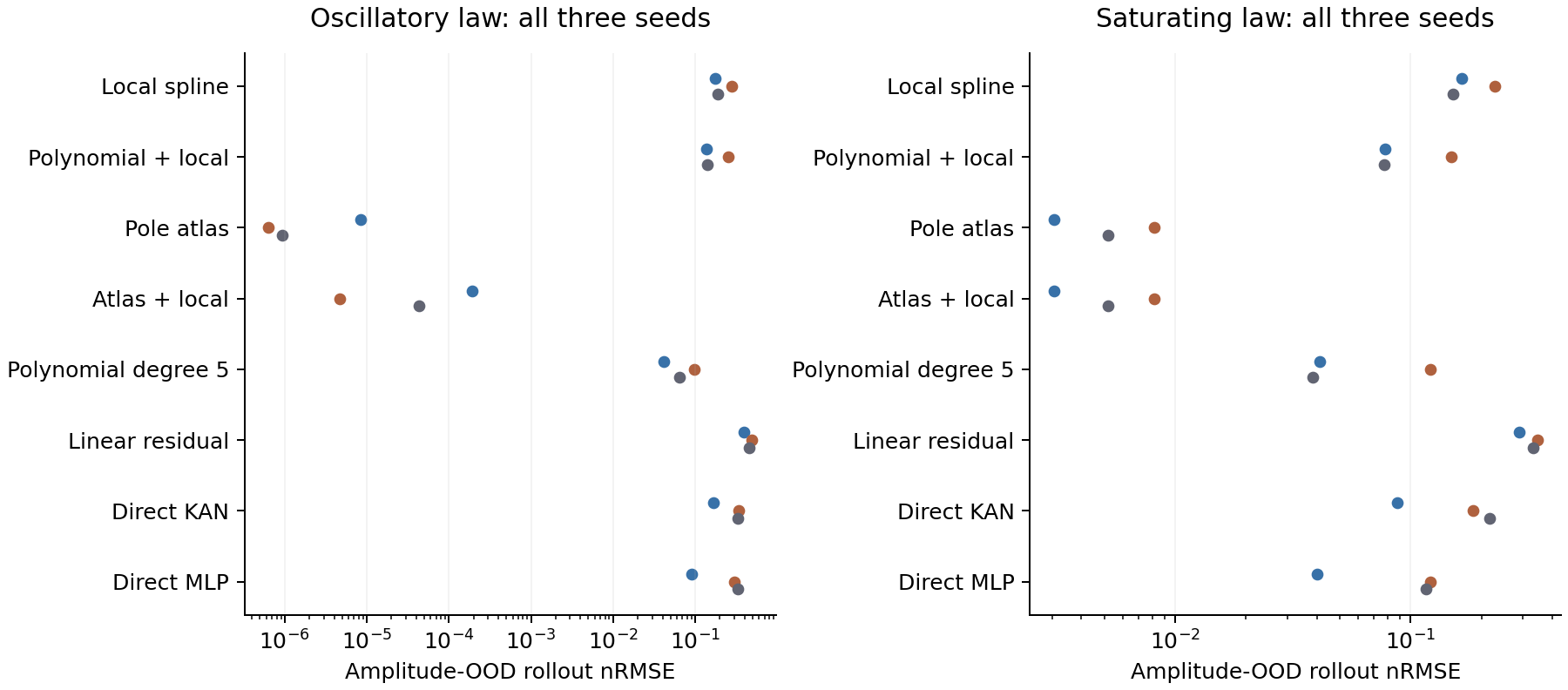
For the matched oscillatory law, the sparse atlas has a worst-seed error of 8.48 × 10⁻⁶ and median 9.29 × 10⁻⁷. This near-exact result is consistent with successful identification of a supplied generating component; it is not evidence of exact extrapolation for an unknown arbitrary law. Adding a local residual worsens the median to 4.27 × 10⁻⁵. More representational freedom is not automatically useful.
For the saturating law, atlas errors are 0.00307, 0.00815, and 0.00520 across the three seeds. The global representation improves on the polynomial and local controls in this panel, even though it cannot exactly express the generating law. However, three deliberately constructed cases cannot establish broad out-of-distribution reliability. Local support helps control where a function changes; it does not provide a reliable extrapolation rule outside the excited state range.
7. Noisy observations and weak identification
A distinct experiment learns both flux and reaction in the same known viscous structure. Its true flux is one-half u squared plus 0.06 sin(4u), and its reaction is 0.25u−0.20u cubed. For a periodic spatial test and a temporal test vanishing at window endpoints, integration by parts gives
The discrete construction uses the adjoint of the discrete temporal difference, rather than assuming that a sampled continuous derivative is the exact discrete adjoint. It combines 25-sample sine-squared temporal windows at stride eight with spatial sine/cosine modes up to eight, giving 2448 weak rows. Eight training trajectories run for 160 steps at amplitude budget 0.65; amplitude-shift evaluation uses 0.95. Independent additive observation noise is scaled to each trajectory standard deviation. The experiment is not pooled with the clean-flux experiment.
| Observation noise | Pointwise atlas | Weak atlas | Weak polynomial |
|---|---|---|---|
| 1% | 0.03844 | 0.001401 | 0.003194 |
| 2% | 0.14635 | 0.006581 | 0.005207 |
Weak fitting markedly improves on pointwise identification in these panels. At 1% noise the weak atlas also improves on the weak degree-five polynomial; at 2% the polynomial is better. Thus robustness arises partly from the observation formulation, not only from the richer dictionary. The complete supplement includes the zero, 0.1%, and 0.5% noise settings as well; the displayed crossover is not suppressed by selecting only the most favorable noise level.
8. Discussion and reproducibility
The central result is architectural placement of learning: a small unknown law can be estimated inside a known evolution model. It is compatible with spline, polynomial, exponential, or neural parameterizations. The best archived method here is a sparse global dictionary, whereas local spline tails fail under substantial amplitude shift. The direct KAN and MLP results support further investigation of structural priors; they do not establish superiority over physics-structured KANs or fully tuned neural solvers.
The development process had access to the synthetic families. No untouched external benchmark is asserted. Each displayed seed has one rollout per shift mode, and correlated temporal samples do not create additional independent tests. Candidate frequencies include the oscillatory generator, the dynamics are one-dimensional and periodic, viscosity is supplied exactly, and observations have no missing-state variables. These are strong favorable conditions. Real experimental identification would need excitation analysis, derivative/observation-model validation, uncertainty propagation, and additional independent systems.
The supplement preserves complete metrics, configurations, active atoms where saved, and source fingerprints. Original runners and dependencies are included. Some neural checkpoints and full rollout trajectories were not stored with these metric files, so the manuscript does not present reconstructed neural movies as archived predictions. Figures are extracted from existing records; no retraining or outcome-driven selection was performed during manuscript preparation.
9. Application boundary and research implication
The resulting design pattern is a solver with a learned material or transport component. It is useful when that component is lower dimensional than the complete dynamics and sufficiently excited by observations. The unmatched saturating law and noisy polynomial crossover are essential tests of that premise. A different physical system would need a newly justified constitutive interface, not merely the same successful dictionary transplanted into it.
10. Conclusion
Known dynamics and unknown constitutive behavior can be separated into a compact learning problem with interpretable parameters. The experiments demonstrate accurate amplitude-shift prediction in a matched dictionary and a useful but imperfect extension beyond that dictionary. They also expose local-tail failures and a noise level where a simpler weak polynomial wins. The transferable lesson is to identify which physical component must be learned and to test its extrapolation mechanism, rather than to infer a universal advantage from a model name.
References
- S. L. Brunton, J. L. Proctor, and J. N. Kutz. Discovering governing equations from data by sparse identification of nonlinear dynamical systems. PNAS, 113(15), 3932–3937, 2016. Source
- D. A. Messenger and D. M. Bortz. Weak SINDy for Partial Differential Equations. arXiv:2007.02848, 2020. Source
- Z. Liu et al. KAN: Kolmogorov–Arnold Networks. arXiv:2404.19756, 2024. Source
- M. Unser and T. Blu. Cardinal Exponential Splines: Part I—Theory and Filtering Algorithms. IEEE Transactions on Signal Processing, 53(4), 1425–1438, 2005. Source