Research manuscript · revised scientific draft
Continuous-Domain Retention in Local Spline Adaptation: Guarantees, Counterexamples, and Sparse Updates
Daniel Schmitter
Abstract
Compact sufficient statistics, unchanged historical predictions, and successful new learning are different properties of an adaptive model. We formalize this distinction for fixed-coordinate cardinal spline corrections to a known physical law. A ridge-regression counterexample shows that exact accumulated statistics need not preserve old predictions. Protecting observed samples likewise permits changes between them. Freezing every coefficient whose basis support intersects a protected interval instead guarantees continuous-domain retention, provided the basis, coordinates, and routing remain fixed. Archived experiments show that this guarantee alone can freeze noisy errors. A sparse one-atom update rule with independent validation combines the support constraint with useful learning on a deliberately sparse synthetic stream. Across twenty confirmation seeds, the mean relative derivative error is 4.99 × 10⁻⁴, compared with 0.0715 for a specified sequential-gradient control; observed protected-region drift is zero. These results demonstrate conditional retention and a bounded sparse-learning mechanism, not unrestricted continual learning, autonomous recursive self-improvement, or unlimited memory.
1. Introduction
A small model that learns locally while leaving established behavior unchanged is an attractive component for adaptive scientific systems. Compact support suggests a way to isolate updates, and accumulated normal equations suggest a way to retain past fitting evidence without replaying raw observations. Neither observation alone proves that an adaptive system will not forget.
This paper separates three claims: preservation of a fixed-feature least-squares objective, preservation of a function on a declared continuous domain, and accurate learning of later tasks. It provides elementary counterexamples, a support-based sufficient condition with proof, and an empirical sequence in which increasingly strong protection first reveals and then reduces a plasticity failure. The experimental contribution is limited to a known carrier with sparse local constitutive defects.
2. Related work
Compact support and coefficient-domain inner products are classical spline tools [1,2]. Sufficient statistics for fixed-feature least squares are also standard linear algebra; retaining them is not a new mathematical guarantee of lifelong learning. Learning without Forgetting uses existing model outputs to constrain adaptation [3], whereas progressive networks preserve prior components and add capacity [4]. These approaches motivate distinguishing what is protected and what is allowed to change.
Our construction protects an entire interval through fixed local supports. It differs from soft distillation penalties and from invariance only at a finite sample set. It does not solve automatic task routing or unrestricted capacity growth. Immutable versions are another valid retention mechanism, but require selecting the right version and retaining its storage. The following experiments update one local model and do not establish a general version-routing system.
3. Architecture and information flow
The adaptation architecture separates a candidate generator from a commit decision. New observations identify eligible local atoms after subtracting the known carrier. Support closure removes every coefficient capable of affecting an already protected interval. A sparse candidate is fitted on one set of profiles and evaluated on distinct validation profiles. Acceptance changes both the coefficient state and the protected-domain mask; rejection leaves both unchanged. Accumulated normal equations are an additional evidence object, not the reason the continuous guarantee holds.
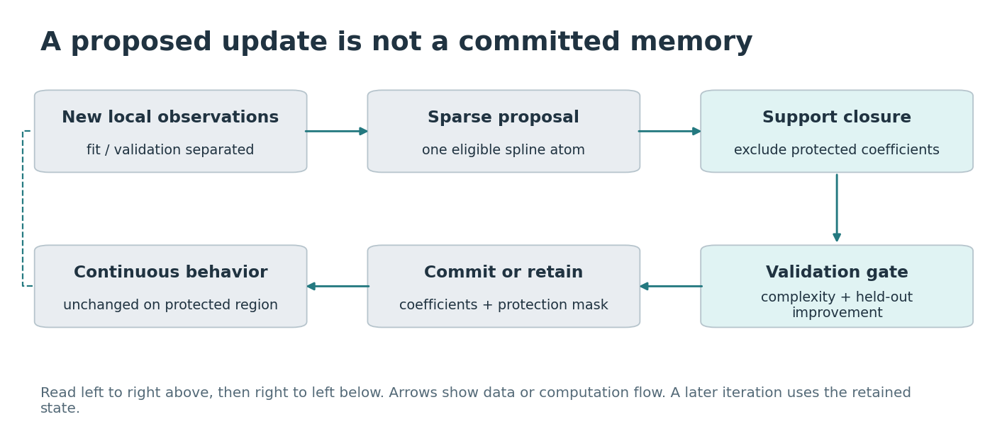
This ordering matters. Protecting a region before a useful update is established can permanently preserve an error. Fitting a dense free subspace can also spread noise into every subsequently frozen degree of freedom. The development sequence tests both failure modes. The successful sparse rule matches the deliberately one-atom innovations, so its excellent error ratio cannot be extrapolated to overlapping or dense changes. Support closure consumes capacity and can eventually leave no admissible update.
4. Three notions of memory
Let a fixed feature vector z(x) define a scalar model. Accumulated normal equations encode all observed squared-loss terms up to an additive constant:
For an unchanged feature map, weighting rule, and ridge coefficient, this is the batch ridge solution on all accumulated observations. It does not preserve the earlier optimum. With one scalar feature equal to one, =1, and first target +1, the coefficient is 1/2 and the old squared error is 1/4. Adding target −1 gives coefficient zero and old error one. Both observations remain exactly represented in G and b. The old prediction worsens despite lossless statistical accumulation.
Similarly, imposing zero update at stored inputs constrains only an evaluation matrix. A compact cubic bump centered between two stored endpoints can vanish at both endpoints and remain nonzero inside the interval. The accompanying numerical fixture uses a centered cubic bump of width 0.12 at x=0.5; its values at zero and one are zero, while its peak is 2/3. Finite pointwise invariance is therefore not continuous-region invariance.
5. Continuous protection
Proposition 1. If the carrier, basis functions, input coordinates, and routing are fixed, then any coefficient update that is zero on S(P) leaves the model unchanged on P. Proof: at any point in P, each changed coefficient multiplies a basis function whose support is disjoint from P; every such contribution is zero. Summing gives zero function change. This is a sufficient condition, not a necessary characterization of all preserving updates.
An alternative continuous test uses the restricted Gram matrix. For continuous basis functions, a zero integral of the squared update on an interval implies pointwise zero throughout that interval:
Continuity proves the implication: a nonzero value would persist on a neighborhood of positive measure and make the integral positive. On interval interiors where derivatives exist, identical functions also have identical derivatives. In floating point, a small quadratic value is only a numerical bound, not exact logical equality. For cubic pieces, four-point cell quadrature exactly integrates the degree-six squared update in real arithmetic.
The support constraint is deliberately conservative. As protected intervals cover the state domain, fewer free coefficients remain and useful adaptation can become impossible. A change to a shared upstream transform can invalidate protection even if local coefficients do not move. Preserving a constitutive law on P also does not preserve every dynamical rollout: a trajectory may leave P and enter a changed region.
6. Sparse adaptation with validation
The deployed correction is additive to a supplied carrier. Each arriving task provides a fitting probe set and an independently generated validation probe set. A candidate update uses only currently unprotected coefficients that are active in the fitting data. The sparse variant fits each eligible single atom by ridge regression and selects the best residual decrease.
Here r is the current residual, n the number of fitting rows, and M the number of eligible candidates. The candidate must have negative extended-BIC difference and at least 5% relative validation-error improvement. On acceptance the coefficient is committed, its task interval is protected through support closure, and fitting statistics are accumulated. On rejection the previous model and protected state are retained. This rule is specialized to sparse defects; a one-atom update cannot represent arbitrary newly encountered behavior.
Derivative observation rows touch at most four neighboring cubic coefficients. Their normal-equation matrix is therefore banded with half-bandwidth three. Storing one symmetric band and the right-hand side takes approximately five doubles per coefficient, or 40K bytes. This is storage for those statistics only: coefficients, masks, metadata, raw validation probes, and audit histories are additional. A dense matrix is not the only alternative; ordinary sparse or banded solvers are essential comparators.
7. Experimental methods
The synthetic law is a known carrier, one-half u squared plus 0.04 exp(0.3u) sin(3.7u), with six localized cardinal-cubic defects. The basis has 121 centers on [−1.5,1.5], spacing 0.025. Nominal defect centers −1.10, −0.68, −0.24, 0.22, 0.67, and 1.08 are snapped to the nearest basis centers; amplitudes are 0.038, −0.031, 0.044, −0.036, 0.033, and −0.040. Each innovation is thus deliberately representable by one atom.
The task stream visits the six regions in order, revisits them in reverse order, and then presents one null region: thirteen blocks. Each block provides four fitting and two validation profiles with 256 spatial samples each. Profiles use sinusoids with randomized phases and local state variation; the carrier contribution is known and subtracted. Observation noise is 2% of the larger of clean residual standard deviation and 0.01. The protected interval has radius 0.21 around a task center.
Four development stages use the same eight seed labels, 20260911 through 20260918: pooled banded statistics; protection of coefficients active at historical samples; continuous region protection with a dense fit over free coefficients; and sparse region-protected updates. These are an informative development sequence, not four independently optimized methods on an untouched test. The sequential cardinal control uses sixty gradient steps per block with a step derived from the largest Gram eigenvalue. A Fourier control is also retained in the full development records.
The final sparse rule was then evaluated on twenty confirmation seeds, 20261011 through 20261030. These numbers identify random seeds, not calendar dates. There are 120 novel-region blocks, 120 revisits, and twenty null blocks, grouped within twenty streams. Derivative error is evaluated against the known true correction. Rollout tests use periodic 96-point dynamics with viscosity 0.04, RK4 step 0.00075, and 160 steps for six initial conditions. Their relative error is normalized by the norm of the true trajectory change from its initial state, not by the trajectory standard deviation used in the constitutive-learning paper.
8. Results
| Method | Derivative error | Retention outcome |
|---|---|---|
| Pooled statistics | 0.02183 | Old-region regression occurs |
| Sample-support protection | 0.04396 | Zero sample drift; region regression remains |
| Continuous region protection | 0.05341 | Zero region drift; accuracy gate fails |
| Sparse region protection | 0.000447 | Zero region drift; sparse learning succeeds |
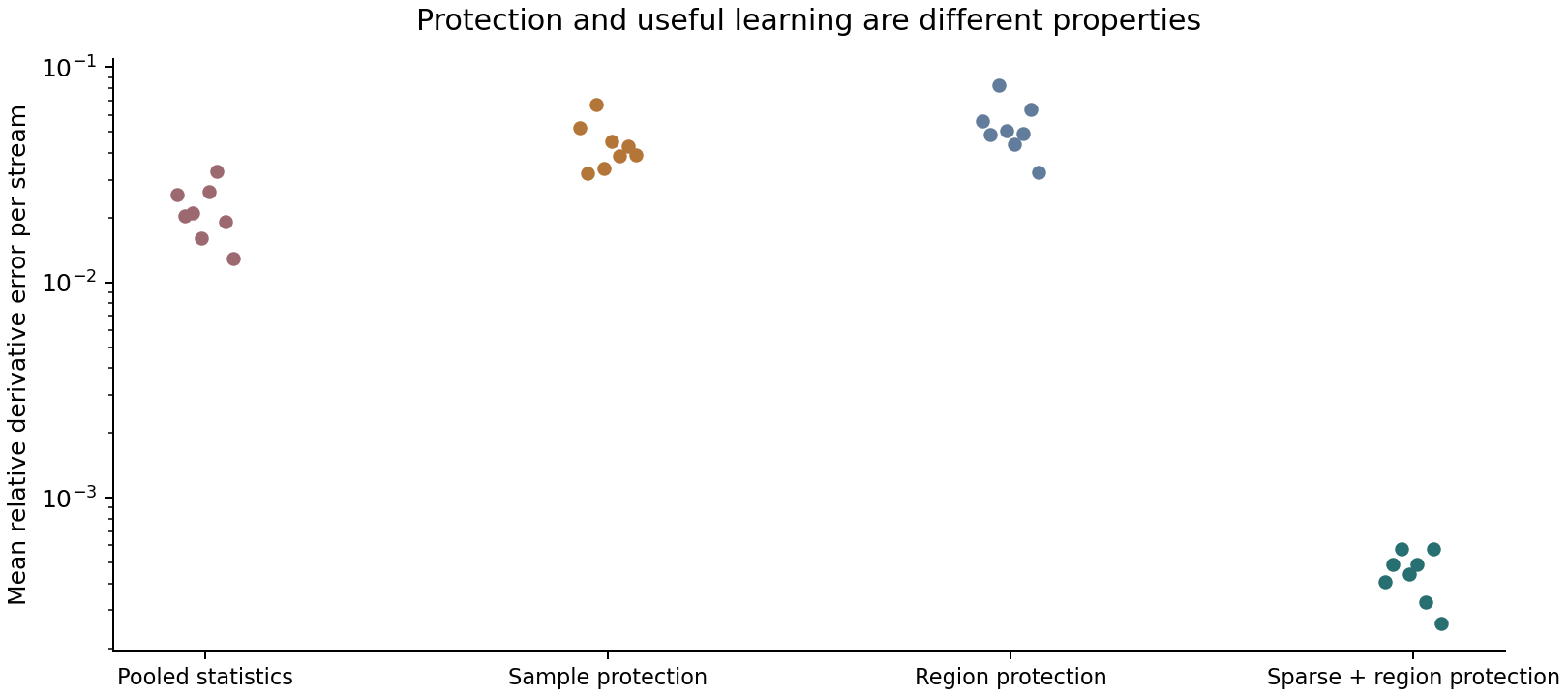
Pooled sufficient statistics retain the fitting contributions but exhibit maximum recorded old-region regression 0.685. Sample-support protection gives zero sampled prediction drift yet maximum region regression 1.378. Continuous protection removes the region drift but yields mean derivative error 0.0534, above the predeclared 0.05 accuracy gate. These failures isolate separate mechanisms: preserving evidence, preserving sampled outputs, and preserving a useful continuous law are not interchangeable.
In the twenty-seed confirmation, sparse protection has mean relative derivative error 0.0004988, versus 0.07151 for the specified sequential control, a ratio of about 143.4. Reported protected-region and sampled drifts are zero. The median rollout error is 0.0001442, compared with 0.3149 for the carrier alone. These numerical gains are conditional on the known carrier, local excitation, aligned single-atom defects, and validation rule. No general continual-learning benchmark or unknown-task-routing evaluation was performed.
The pooled-statistics audit also contains a numerical failure worth retaining: Gram and right-hand-side discrepancies are near 10⁻¹⁵, but a coefficient comparison around 1.5 × 10⁻¹⁰ exceeds its 10⁻¹¹ threshold. Near-singular or regularized solves can amplify small matrix differences. We therefore do not report that every numerical audit passed merely because the statistics themselves agree closely.
9. Discussion and reproducibility
A retention guarantee is meaningful only after specifying the protected function, domain, and fixed coordinates. It says nothing by itself about whether the current prediction is correct. The dense protected stage makes that distinction concrete by preserving noisy errors. Sparse validated proposals work well because the experiment supplies exactly the sparse structure they assume. Broader defects, overlapping regimes, drifting coordinates, imperfect carriers, and exhausted free support remain unresolved.
The fixed-feature batch-equivalence statement assumes fixed regularization. The experimental runner rescales a ridge term with the accumulated Gram diagonal, so its entire update sequence should not be equated with one fixed-ridge trajectory. Likewise, the audit harness keeps raw evidence for verification; compact statistic storage is not a measurement of the full experimental process footprint. The supplement includes complete stage records, source hashes, and executable counterexamples. A JSON field called restricted continuous L2 drift stores the integrated squared difference, not its square root; both are zero in the stated protected tests.
The work provides a small verified adaptation primitive, not recursive self-improvement. A larger system would still need to choose tasks, gather informative observations, route contexts, budget capacity, validate safety-relevant behavior, and assess cumulative uncertainty. Immutable versions or disjoint modules can preserve old functions under different conditions, but their storage and routing costs cannot be omitted.
10. Application boundary and research implication
The deployable abstraction is an auditable local revision with a stated invariant. It could sit inside a larger learning system, but task discovery, coordinate changes, routing, and capacity replenishment remain outside the tested mechanism. A fixed-coordinate retention guarantee is valuable precisely because it is smaller and more verifiable than an unrestricted promise of no forgetting.
11. Conclusion
Continuous support protection gives a simple exact retention condition for fixed-coordinate local spline models. Counterexamples rule out stronger claims based only on sufficient statistics or historical samples. In a deliberately sparse constitutive-learning stream, combining the support constraint with sparse validated proposals retains protected behavior while accurately learning new local defects. The result is a conditional and auditable building block for adaptation, with explicit limits on plasticity and system-level interpretation.
References
- C. de Boor. A Practical Guide to Splines. Revised edition. Springer, 2001. Source
- A. Badoual, D. Schmitter, and M. Unser. An Inner-Product Calculus for Periodic Functions and Curves. IEEE Signal Processing Letters, 23(6), 878–882, 2016. Source
- Z. Li and D. Hoiem. Learning without Forgetting. arXiv:1606.09282, 2016. Source
- A. A. Rusu et al. Progressive Neural Networks. arXiv:1606.04671, 2016. Source