Research manuscript · revised scientific draft
Blockwise Reverse-Mode Differentiation and Predictive-Coding Relaxation: An Implementation-Level Comparison
Daniel Schmitter
Abstract
A local autodifferentiation graph does not imply a learning rule without reverse credit propagation. We analyze two archived implementations: a blockwise vector-Jacobian sweep and a predictive-coding relaxation system. The first is exactly the reverse-mode chain rule under fixed forward states and parameters, despite detaching activations between blocks. Small CPU-only tests compare the original update functions against a global backward pass and independent directional finite differences. A saved two-seed, sixty-epoch CIFAR-100 comparison reaches mean accuracy 0.6905 for the blockwise sweep and 0.6916 for global backpropagation. The second implementation performs genuine iterative hidden-state relaxation; its finite-step gradients differ substantially in early layers, and the retained convolutional experiment reaches 0.3993 accuracy versus 0.5447 for the matched mean-squared-error backpropagation control. We derive the distinction, report the complete selected diagnostic panels, and explain why accuracy differences between exact-gradient implementations cannot establish a new learning principle. The contribution is mechanistic identification and reproducible diagnostics, not a universally superior local learning algorithm.
1. Introduction
Local learning can refer to local observations, local parameter updates, adjacent-layer error messages, or separate software graphs. These are different properties. A computation may be written using only per-block automatic differentiation while its credit signal still depends on a reverse traversal of the entire network. Conversely, an iterative local-state system may approximate that credit signal without reproducing it after a finite number of steps.
We analyze both mechanisms in executable project code. The purpose is not to dismiss local computation: blockwise organization can be useful for memory scheduling and modular implementations. It is to determine which algorithm is actually being compared before assigning biological or optimization significance to a result.
2. Related work
Predictive-coding systems have been related to backpropagation under specific dynamics and limiting conditions, including arbitrary computation graphs [1]. Related work studies exact implementations under particular update schedules [2]. These results do not imply that every finite relaxation or every detached software block is a distinct biological learning rule. The present study identifies the actual dependencies of two implementations and checks their derivatives directly.
3. Architecture and information flow
Two computational graphs are compared, not two names for the same code. In the blockwise sweep, forward activations are retained and the terminal loss derivative moves backward through local Jacobian products. All parameter updates occur after the sweep. In the relaxation system, hidden values move for a finite number of iterations before local energy derivatives are evaluated. Its additional state and iteration budget are part of the learning computation.
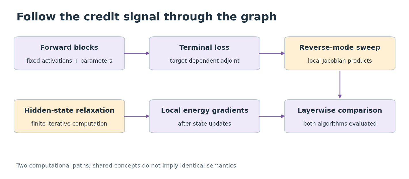
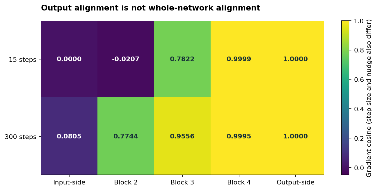
A block boundary can be a useful software scheduling boundary without being a biological credit-assignment boundary. Exact equality to backpropagation requires matching stochastic states and update order. Conversely, a relaxation residual or output-layer gradient match is insufficient to characterize the early layers. The observed layerwise cosine profile exposes that gap and explains why final accuracy alone is not a diagnostic of the proposed mechanism.
4. Blockwise reverse adjoints
Let each block map its incoming activation to its output using local parameters, and let the loss depend on the final output. Holding all forward activations and parameters fixed during differentiation gives
Proposition 1. A reverse traversal evaluating these local vector-Jacobian products yields the same parameter derivatives as global reverse-mode differentiation. Proof. At the last block the statement is the chain rule for the loss composed with that block. Substituting the resulting incoming adjoint into the preceding block applies the same rule to the next composition. Backward induction reaches every parameter. Detaching the stored activations changes automatic graph bookkeeping but not these derivatives when the incoming adjoint is explicitly supplied.
The archived blockwise runner implements this recurrence using autograd.grad on each output with respect to its input and parameters. It passes the returned input gradient to the next block in reverse order. For cross-entropy, the terminal adjoint is softmax probability minus one-hot target, divided by batch size. All blocks update only after the sweep. Calling this gradient-free would be incorrect. It uses the same parameter Jacobians, global target information, and reverse dependency chain.
Equality assumes identical forward states, stochastic realizations, loss scaling, and parameter values. Recomputing dropout differently, updating weights mid-sweep, changing normalization state, or comparing different losses can invalidate it. A detached implementation also does not automatically save activation memory: this runner retains each local input-output graph until its reverse use.
5. Finite predictive-coding relaxation
The separate convolutional prototype defines hidden value nodes and adjacent-layer prediction errors. After a feedforward initialization, it fixes the input, nudges the output toward its target, and descends a sum of local prediction energies with respect to hidden values while holding weights fixed. It then differentiates that energy with respect to weights at fixed values.
This is an iterative state computation, not the one-pass adjoint recurrence. Its result depends on the nudge beta, step size eta, number of iterations T, scaling of the energy, and convergence. In the source the energy is averaged over the batch, which also scales the hidden-state descent step. A small printed residual does not establish accurate gradients in all blocks; its magnitude depends on those conventions.
6. Experimental methods
We inspect the complete CIFAR-100 blockwise runner and the convolutional relaxation and alignment runners, leaving originals unchanged. The saved CIFAR-100 panel has two seeds, sixty epochs, four convolutional blocks of widths 64, 128, 256, and 512, batch normalization, rectification, pooling, and a 100-class head. Both modes use the same source-level architecture and Adam schedule. We report both seeds rather than selecting the favorable run; exact historical random-state equality and bitwise hardware execution are not established by the compact metrics file.
A new bounded CPU-only test extracts the original global and local step functions without running their data loader or training loop. It uses three deterministic tanh/linear blocks of widths 4, 7, 5, and 3, eleven examples, three seeds, and binary32 and binary64 arithmetic. Image normalization is replaced by identity because these are vector fixtures. It measures full-gradient relative error, cosine, loss difference, and an independent centered directional finite difference. No image training or hyperparameter search is performed.
For genuine relaxation, the retained eighteen-epoch CIFAR-10 panel uses four strided tanh convolutional layers, fifteen hidden-state steps, rate 0.1 and nudge 0.2. Cross-entropy and squared-error backpropagation controls are reported separately. The associated five-configuration alignment diagnostic holds untrained weights fixed and compares each parameter block with the squared-error reference on one 512-example augmented batch. It is an exploratory diagnostic, not five independent experiments.
7. Results
| Experiment | Method | Recorded accuracy |
|---|---|---|
| CIFAR-100, seed 0 | Global / blockwise | 0.6913 / 0.6880 |
| CIFAR-100, seed 1 | Global / blockwise | 0.6919 / 0.6931 |
| CIFAR-10 relaxation | Backprop cross-entropy | 0.5411 |
| CIFAR-10 relaxation | Backprop squared error | 0.5447 |
| CIFAR-10 relaxation | Finite-step predictive coding | 0.3993 |
The CIFAR-100 means differ by 0.0011 in favor of the global implementation, with opposite signs in the two paired runs. This small descriptive panel does not establish equivalence within a predeclared statistical margin or an intrinsic advantage. More fundamentally, both update formulas implement the same exact derivative under the proposition’s conditions. Divergent long-run outcomes must therefore be attributed to execution, randomness, numerical propagation, or changed conditions rather than a new derivative rule.
All six bounded gradient comparisons meet the declared relative-error tolerances: less than 10⁻¹² for binary64 and 10⁻⁵ for binary32. The supplement retains every measured value and finite-difference discrepancy. This validates the extracted update mechanism on deterministic blocks; it does not certify every convolutional or recurrent implementation in the larger archive.
In the fifteen-step relaxation diagnostic, the five gradient cosines are 0.0000, minus 0.0207, 0.7822, 0.9999, and 1.0000 from the input-side to output-side parameters. At 300 steps, rate 0.3 and nudge 0.05, they become 0.0805, 0.7744, 0.9556, 0.9995, and 1.0000. Better agreement near the output does not show that the entire network receives the correct derivative. The saved diagnostic lacks gradient norms, so cosine alone cannot establish magnitude agreement; its zero values may also involve tiny gradients.
8. Discussion
The study supports two different conclusions. A block-local software sweep can reproduce backpropagation exactly. A finite predictive-coding relaxation can fail to do so, particularly in early layers, and can underperform in the retained task. Neither conclusion resolves biological plausibility or rules out useful alternative local dynamics. Those require their own information, timing, and resource models.
Runtime advantages are possible for an implementation even when its mathematics is unchanged, but they need matched end-to-end timing and memory measurements. The inspected final-accuracy file does not supply that evidence. Likewise, identical derivatives do not themselves explain claims of different implicit regularization. The complete named results, source fingerprints, and independent small tests make these distinctions reproducible without retraining a vision model.
9. Application boundary and research implication
The practical contribution is an implementation-level test of learning semantics. A future memory or hardware advantage could exist even when the derivative is unchanged, but it must be measured as such. The present record supports a verified reverse-mode decomposition and a finite-relaxation failure, not a general replacement for backpropagation.
10. Conclusion
Locality of software graphs and locality of credit assignment should not be conflated. The audited blockwise sweep is reverse-mode differentiation; the relaxation system is a different finite computation whose early-layer agreement is poor in the retained diagnostic. Identifying those mechanisms produces a stronger scientific statement than an unsupported assertion that local learning universally replaces or surpasses backpropagation.