Research manuscript · revised scientific draft
Operator-Aware Residual Assimilation: Improved Field Recovery and a Failure of Trajectory Transfer
Daniel Schmitter
Abstract
An operator-informed correction can improve a reconstructed field without improving its downstream use. We study a matrix-free cardinal residual fitted to sparse observations with a coefficient-weighted derivative energy. On 134 previously unopened PDEBench Darcy fields, 32 observations per 128-by-128 field reduce mean blind relative error from 0.02771 for a selected cosine residual to 0.01674, with 120 paired wins. The same basis without conductivity weighting is less accurate, isolating a contribution from the physical metric. A discrete strong-operator mismatch nevertheless worsens. In a separate six-stream turbulence test, a divergence-informed correction improves global field error but worsens every particle rollout. We formulate the quadratic mechanism and output-error distinction explicitly. The contribution is a bounded sparse-assimilation result and a falsifying downstream test, not a general PDE solver or forecast capability.
1. Introduction
Scientific learning may be judged by field accuracy, equation residual, or a downstream decision. These objectives are related but not interchangeable. We examine whether known spatial conductivity improves sparse reconstruction of an observed steady field, then whether a divergence correction that improves instantaneous velocity improves trajectories. These are separate datasets and estimands; the negative result is not averaged away by the positive one.
2. Related work
PDEBench supplies the Darcy data [1], but our target-field sensor access defines assimilation rather than its ordinary unseen-input prediction task. Turbulence fields originate from JHTDB [2]. Physics-informed neural networks [3] provide one archived comparator, not the only classical or learned alternative. Derivative-energy quadratic forms are established approximation tools [4]; the measured contribution concerns a coefficient-aware residual and a fixed validation rule.
3. Architecture and information flow
The assimilation model is a correction layer around a supplied numerical prior, not a neural operator trained to forecast unseen targets without sensors. Sparse observations fit a scale and residual; a small validation set selects regularization or rollback. Matrix-free contractions expose the physical derivative energy without requiring a dense coefficient normal. The dynamic follow-up uses a separate velocity dataset and particle integrator to test a different output.
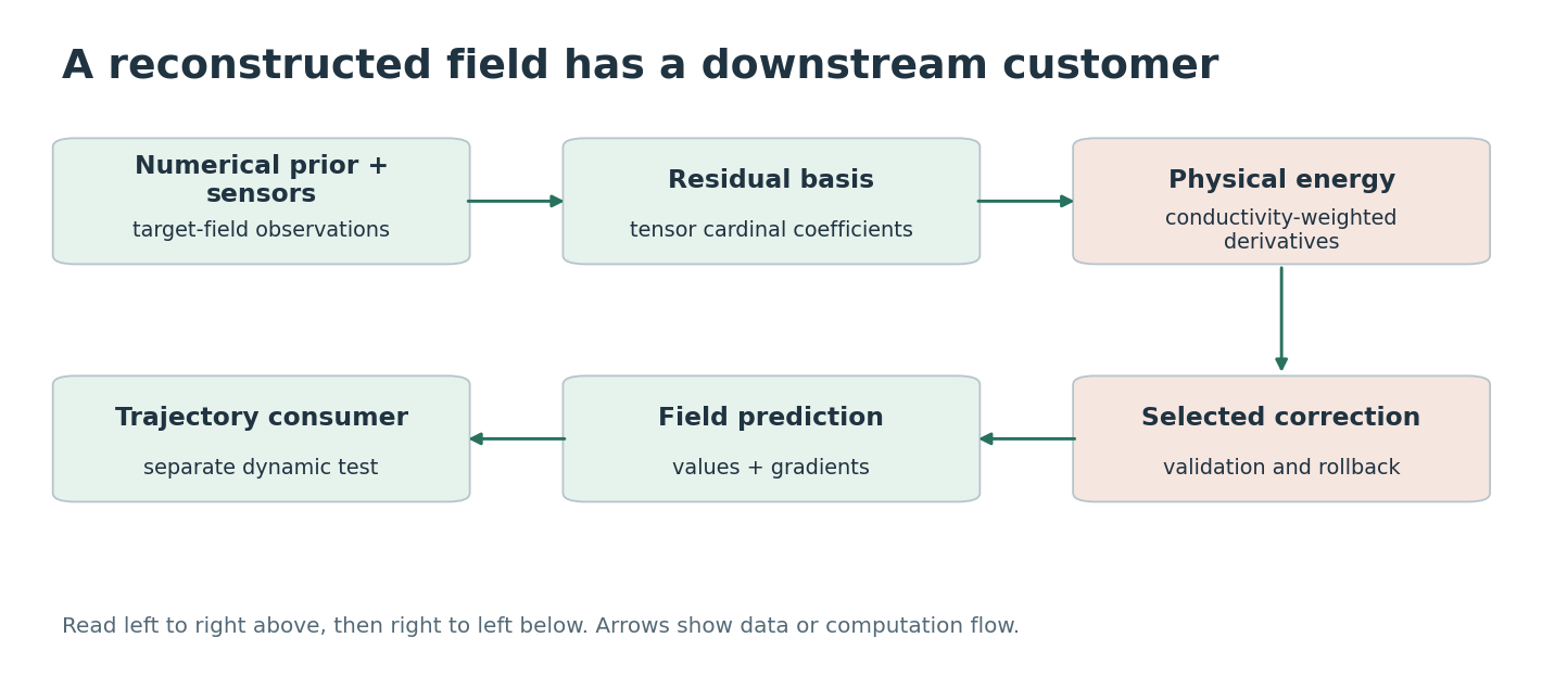
Three error geometries coexist. Sensor loss measures values at observed points. The operator energy weights derivatives across a field. The particle solver samples velocities along trajectories that change when the field changes. A lower first or second quantity cannot in general order the third. This explains why the Darcy ablation and the turbulence failure can both be genuine results without contradicting the quadratic algebra.
4. A conditional quadratic correction
Let u_0 be a supplied numerical prior, y a sensor vector, and S the sensor operator. The corrected field is a fitted scalar multiple of u_0 plus Bc, where B is a tensor cardinal basis. After fitting the scalar on fitting sensors, the coefficient objective is
Tensor basis and derivative contractions apply the normal and its adjoint without forming a dense coefficient matrix. The implementation samples the supplied conductivity bilinearly at tensor Gauss nodes. Positive quadrature weights and nonnegative conductivity produce a positive semidefinite energy normal; positive ridge makes the full finite-dimensional system positive definite. Exact adjointness of this discrete form does not imply exact integration of an arbitrary heterogeneous continuum coefficient.
The code uses trace-matched energy scaling, a tenfold boundary trace scale, relative ridge 10⁻⁴, and Jacobi-preconditioned conjugate gradients. Boundary samples penalize rather than exactly enforce a boundary condition. This is not a full Darcy-residual minimization: it regularizes the correction while relying on a supplied finite-volume prior and observed target values. Selection includes rollback and zero energy.
5. Field error and trajectory error
Let true and approximate trajectories start at the same point. If the true velocity is spatially L-Lipschitz and the velocity discrepancy is uniformly at most epsilon on the relevant domain and times, adding and subtracting true velocity on the approximate path gives e-prime at most L e plus epsilon. Integration yields
For L zero, the limit is epsilon times t. Global mean-square field error does not supply the required pathwise uniform bound. Divergence also does not control all errors: adding a constant velocity changes trajectories while preserving divergence. Thus neither diagnostic alone is a trajectory guarantee. This elementary stability argument identifies the missing quantity without asserting that any observed regression must harm a path.
6. Experimental methods
The Darcy study uses 64 development rows and 134 later rows of a local PDEBench shard, with row ranges and hashes retained. Each field has supplied 128-by-128 conductivity and 32 fixed solution sensors, or 0.195% of cells. A ten-by-ten coefficient tensor augments the same arithmetic-face finite-volume prior. Eight sensors select rollback, data-only correction, or one of seven energy strengths, followed by refitting on all 32. Blind metrics exclude sensor cells.
Controls are a fitted scalar prior, a selected cosine residual with ranks 8, 16, and 32 and three ridge values, the same cardinal basis without energy, and isotropic-energy regularization. Gradient error is conductivity weighted. A separate discrete strong-operator mismatch is retained despite an interface convention not fully matching the benchmark. No central model is trained across target fields.
The turbulence follow-up freezes trilinear-plus-cardinal divergence correction before six new five-frame streams. Each uses an eight-cubed sensor lattice and 64 fixed particles integrated by RK4. Endpoint and all-time trajectory errors compare correction with uncorrected interpolation. A PINN-plus-residual path remains as a control; beating that path is insufficient if simple interpolation already does better.
7. Results
| Method | Blind relative error | Weighted gradient | Strong mismatch |
|---|---|---|---|
| Scalar prior | 0.05444 | 0.09903 | 0.5565 |
| Cosine residual | 0.02771 | 0.11181 | 0.9359 |
| Cardinal data only | 0.01922 | 0.10606 | 1.5131 |
| Cardinal isotropic | 0.01853 | 0.10145 | 1.4735 |
| Cardinal conductivity | 0.01674 | 0.08859 | 1.3556 |
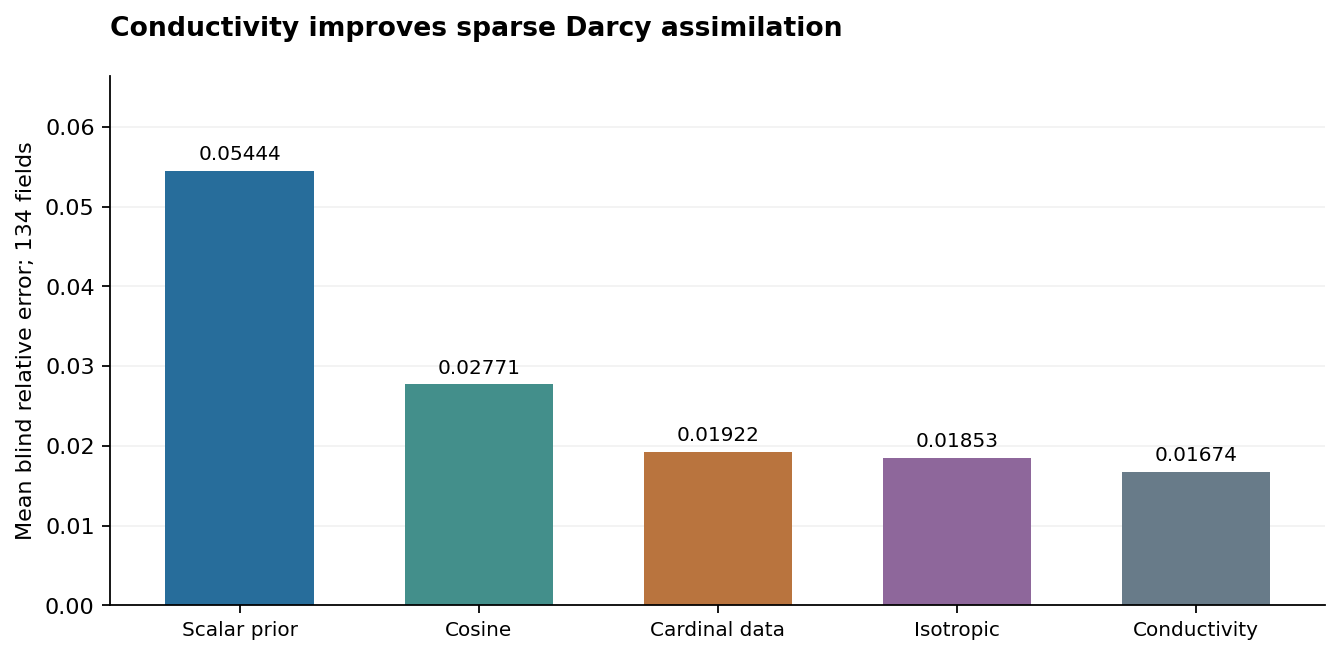
Conductivity weighting wins 120 of 134 blind-value comparisons against cosine. Mean reduction is 39.57% against cosine, 12.90% against the same data-only basis, and 9.65% against isotropic energy. Positive energy is selected in 66 fields, zero energy in the others. Strong mismatch is worse than cosine and the scalar prior; this is not a recovered strong-form solution.
Recorded checks cover symmetry, positivity, trace, zero rollback, and solve residuals. Worst deployed relative solve residual is 9.98 × 10⁻⁹. The research loop, including every candidate and control, takes about 0.937 seconds per field and peaks at 428 MiB RSS. This is not the latency of only the final selected solve.
Across six turbulence streams, global blind velocity improves on all thirty frames, while endpoint and all-time errors worsen on every stream. Median paired deteriorations are 7.34% and 6.56%; median endpoint relative error changes from 0.12224 to 0.13036. A static sensor holdout selects full correction throughout and reproduces the failure. A subsequent material-coherence normal also fails to reverse it. No successful trajectory-transfer claim follows.
8. Discussion
The Darcy result supports target-conditioned assimilation with a meaningful coefficient-aware ablation, not forecasting without sensors. The turbulence result shows why deployment must be scored on its actual output. Dataset-specific discretization, a single shard, and six dynamic streams constrain generalization. Matched classical assimilation controls and new systems would be needed for a broader claim.
All frozen outcomes and source identities are preserved. No simulation, sensor acquisition, or parameter search was added for this reconstruction. The strongest transferable lesson is methodological: compile trustworthy structure, then test its relationship to the functional that matters. A lower physical penalty does not substitute for that final test.
9. Application boundary and research implication
A strong application would make the consumed functional part of model selection while preserving an independent final evaluation. For steady assimilation, that may be a field or flux. For transport, it may be a flow map or hitting event. The tested architecture improves one such objective and fails another; its scope is more informative than a generic claim that adding physics always helps.
10. Conclusion
A variable-coefficient derivative Gram improves sparse steady-field assimilation in the tested setting. Physical regularization does not automatically improve trajectories. Observation access, the represented operator, and the consumed output must be analyzed together.
References
- M. Takamoto et al. PDEBench: An Extensive Benchmark for Scientific Machine Learning. NeurIPS Datasets and Benchmarks, 2022. Source
- Johns Hopkins Turbulence Databases. Dataset descriptions and access documentation. Source
- M. Raissi, P. Perdikaris, and G. E. Karniadakis. Physics-informed neural networks: A deep learning framework for solving forward and inverse problems involving nonlinear partial differential equations. Journal of Computational Physics 378, 686–707, 2019. Source
- A. Badoual, D. Schmitter, and M. Unser. An Inner-Product Calculus for Periodic Functions and Curves. IEEE Signal Processing Letters 23(6), 878–882, 2016. Source