Research manuscript · revised scientific draft

Mergeable Parameter-Dependent Objective Summaries for Stable Scalar Dynamics

Daniel Schmitter

Abstract

A compact learning record can preserve a specified family of later objectives without reconstructing its input samples. We study this distinction for a stable first-order filter with an unknown time constant and a fixed observed target. Three parameter-dependent response functions determine terminal state and squared loss for any incoming state. Their chronological composition yields a fixed-node summary whose merge operation introduces no additional interpolation error in exact arithmetic; first-derivative Hermite data obey the same property. For bounded inputs and targets, we derive a Chebyshev interpolation bound for mean loss that is independent of record length on a fixed time-constant range. A six-seed synthetic panel compares linear, natural cubic, Hermite, and Chebyshev representations at equal scalar budgets. A 32-scalar-per-function Hermite summary meets all 108 record/version checks, while a same-budget Chebyshev summary is substantially more accurate. In a separate million-sample checkpoint panel, all four Hermite/Chebyshev storage-precision arms meet the prescribed error budget, with serialized float32 objects of 438 bytes. This is compression of a restricted objective family, not arbitrary history, unrestricted recurrent learning, or a spline-specific superiority result.

1. Introduction

A sensor history is often retained because a parameter will be reconsidered later. Keeping only today’s fitted parameter removes that freedom; keeping every sample may exceed the storage or communication budget. An intermediate object can preserve how a declared loss changes across the admissible parameter domain. This paper asks when such an object can be merged across time blocks without repeatedly accumulating approximation error.

We use a scalar stable filter to isolate that question. The proposed summary consists of classical affine/quadratic block statistics represented as functions of log time constant. Our contributions are an explicit analysis of fixed-node and first-jet merging, a bounded-input approximation guarantee uniform in record length for mean loss, and equal-storage comparisons with strong non-spline controls. The resulting capability is narrow but operational: after capture, one may change the time constant and incoming state while retaining the same observed targets.

2. Related work

Approximate sufficient statistics are an established route to repeated learning without raw-data scans. PASS-GLM, for example, constructs polynomial approximate statistics for generalized linear model inference [1]. Our dynamic block retains an incoming-state dependence and a chronological composition law rather than an independent-observation GLM objective. This distinction specifies the problem; it does not make sufficient-statistic compression itself new.

Chebyshev interpolation of analytic functions has classical geometric convergence bounds [2]. Hermite interpolation and value/derivative jets are also classical [3]. The comparison here charges each derivative as a stored scalar and includes ordinary global polynomial interpolation. We do not infer spline superiority from a favorable comparison with linear interpolation, nor count parameter nodes as independent experimental replications.

3. Architecture and information flow

Capture evaluates a small set of parameter-dependent block functions rather than selecting one final parameter. Each block carries its incoming-state dependence, so later blocks can be composed in time order. The serialized object stores approximations of those functions. At query time the recipient supplies a time constant and initial state and obtains a terminal state and objective value without replaying interior samples.

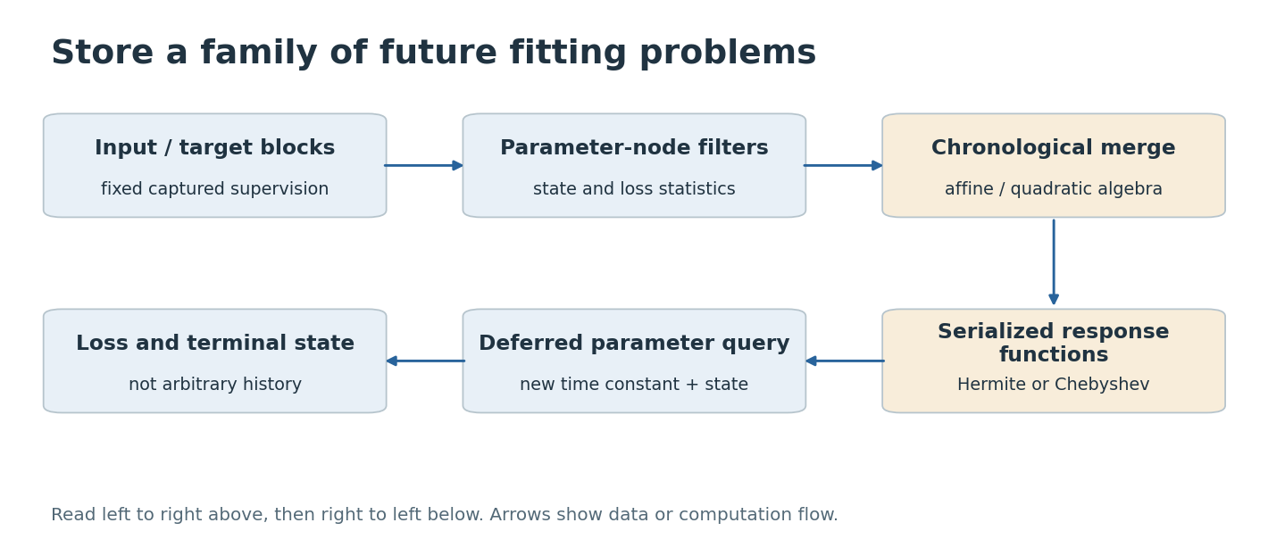
Store a family of future fitting problems. Boxes distinguish supplied information, fitted components, and the quantity evaluated. Arrows show computation or data dependence, not a newly trained deep network.

The merge identity relies on common parameter nodes and on applying the exact block algebra at those nodes. Hermite derivatives are carried by the product rule; they are not free extra observations. A balanced tree may change floating-point summation, but it does not introduce a new real-arithmetic projection at each level. Changing the nodes or replacing nodal algebra with a general projection removes that argument.

4. A block as a parameter-dependent quadratic objective

For a block of N observed input-target pairs, let q depend on the queried time constant and sample interval. The filter starts from a supplied state s. Its zero-initial-state response is denoted z_i^0, with i running from one through N.

q=e^{-\Delta t/\tau},\quad z_i=qz_{i-1}+(1-q)x_i=q^is+z_i^0,\qquad A=q^N,\quad B=z_N^0,\quad P=\sum_{i=1}^Nq^{2i}.

H=\sum_{i=1}^Nq^i(z_i^0-y_i),\quad R=\sum_{i=1}^N(z_i^0-y_i)^2,\qquad z_N=As+B,\quad J_N(s,\tau)=Ps^2+2Hs+R.

Only B, H, and R depend on observations; A and P follow from timing, length, and the query. The implementation retains H/N and R/N for numerical scaling, with N stored as metadata. Thus the number of response functions is fixed even though their approximation across the parameter domain remains a nontrivial task. A new target sequence would in general require cross-products that this object does not contain.

5. Composition and interpolation

For consecutive blocks one and two, substitute the first terminal state into the second loss and add the first loss. The unnormalized statistics compose as follows.

\begin{aligned}A_{12}&=A_2A_1,&B_{12}&=A_2B_1+B_2,\\P_{12}&=P_1+A_1^2P_2,&H_{12}&=H_1+A_1(P_2B_1+H_2),\\R_{12}&=R_1+P_2B_1^2+2H_2B_1+R_2.\end{aligned}

Proposition 1 (fixed-node merging). Suppose every block is represented by values at the same parameter nodes, and the merge evaluates the displayed algebra at those nodes before applying the same interpolant. In exact arithmetic, any parenthesization preserving chronological order produces the same final nodal values as direct accumulation. The final off-node error is the interpolation error of the entire record, not a separate projection error added at each merge.

Proof. Evaluation at a fixed node preserves addition and multiplication. At each node the merge therefore equals the exact block-composition law, which is associative because it represents composition of affine state maps and addition of their quadratic losses. Induction over a merge tree gives the direct whole-record value at every node. Interpolating identical node arrays yields identical response functions. Floating rounding, changed nodes, and approximate nodal statistics are outside this assertion.

The statement extends to Hermite values and first derivatives because a first jet multiplies by the product rule. This permits equal-budget comparison using half as many nodes and a value/derivative pair at each node. The property is not shared by arbitrary function-space projection: on the interval [−1,1], $L^2$ projection onto linear polynomials maps u squared to 1/3 and u cubed to 3u/5, so projecting intermediate products need not preserve the final result.

(f,f')\,(g,g')=(fg,f'g+fg'),\qquad P\big(P(u^2)P(u)\big)=u/3\ne3u/5=P(u^3).

6. A record-length-independent mean-loss bound

Assume bounded observations with absolute input at most X and absolute target at most Y. Parameterize log tau as c+a xi on the real interval xi in [−1,1]. On a Bernstein ellipse of parameter rho greater than one, suppose beta defined below is less than pi/2. Then the complex step w has positive real part, and the stable convolution is uniformly bounded in record length.

a=\tfrac12\log(\tau_{\max}/\tau_{\min}),\quad \beta=\tfrac a2(\rho-\rho^{-1})<\pi/2,\quad C=\sec\beta,\qquad w=\Delta t\,e^{-c-a\xi},\quad \frac{|1-e^{-w}|}{1-e^{-\operatorname{Re}w}}\le C.

The last inequality follows by integrating exp(−tw) from zero to one and using the ratio of the modulus of w to its real part. Summing the resulting geometric convolution gives absolute zero-state response at most CX. Consequently B, H/N, and R/N are analytic on the ellipse and bounded respectively by CX, CX+Y, and the square of CX+Y. The square defining R is the analytic complex square, not a squared modulus.

F_d=\frac{4\rho^{-d}}{\rho-1},\qquad |B-\widehat B|\le F_dCX,\qquad |J_N/N-\widehat J_N/N|\le F_d\left[2S(CX+Y)+(CX+Y)^2\right],\quad |s|\le S.

Proposition 2. The displayed bounds hold for degree-d Chebyshev interpolation of the three functions, with A and P evaluated exactly. Proof. Apply the classical analytic interpolation bound [2] to each function and combine the H and R errors in the mean-loss expression. The state contribution involving P and terminal contribution involving A introduce no interpolation error. None of the resulting constants depends on N. The proposition does not cover finite-precision checkpoints, unbounded observations, or total loss without its factor of N.

If a uniform objective approximation error is epsilon and its minimizer is global, evaluating the true objective at that minimizer incurs regret at most twice epsilon relative to the true global minimum. This follows by inserting and subtracting the approximate objective at both minimizers. Our numerical optimizer uses a grid followed by a local bounded search; it is not a certified global minimizer, so observed optimization regret is reported separately.

7. Experimental methods

The short-record panel has six confirmation seeds 937101–937106, two lengths 8192 and 65536 over eight seconds, and three target regimes. Inputs combine a chirp, independent Gaussian fluctuations, and random steps, normalized to RMS one. Targets are a filter with time constant 0.037 seconds; a continuous-state switch from 0.015 to 0.12 seconds halfway through; or tanh of a 0.055-second filtered input. Target Gaussian noise has standard deviation 0.02. The fitted family is always a constant-parameter linear filter over time constants [0.002,0.2] seconds, including under misspecification.

Linear and natural cubic tables use uniformly spaced log-time nodes. Cardinal cubic Hermite uses half as many nodes, retaining exact analytic sensitivities. Chebyshev-Lobatto interpolation uses the full scalar budget. Budgets are 32 or 64 binary64 scalars per function. Every record has a direct summary and sequential and balanced merges of 32 blocks. All versions are serialized before 257 independently drawn log-uniform queries plus both endpoints, each at incoming states −2, zero, and two.

Each representation must pass all 108 record/version checks: normalized terminal-state and mean-loss errors and raw-objective regret no greater than 0.0001; no material negative quadratic Schur value; and at most 2048 serialized bytes. Optimization uses 65 log-uniform trials followed by bounded search around the best trial. Full-data compiled filtering is the query-time comparator. Encoding, merging, decoding, and break-even costs remain separate from warm-query timing.

A separate six-seed panel, 938101–938106, streams 1,048,576 samples at interval 0.001 seconds. Bounded inputs combine a chirp of amplitude 0.4, Rademacher noise of amplitude 0.3, and bounded chunkwise steps of amplitude 0.3. Targets use a constant 0.037-second teacher or a continuous-state switch from 0.012 to 0.15 seconds, with bounded noise of amplitude 0.02. Each 1024-sample merge is serialized to float32 or float64 and restored. All calculations remain float64. Four prefixes are queried after capture; reference streams are regenerated with matching hashes. This tests storage rounding, not low-precision processing hardware.

8. Results

Equal-storage objective summaries. Each row contains 108 final versions from 36 related records; bytes include metadata.
Representation	Scalars/function	Passes	Worst mean-loss error	Bytes
Linear	32	0/108	3.64 × 10⁻⁴	802
Linear	64	0/108	8.80 × 10⁻⁵	1570
Natural cubic	32	45/108	9.70 × 10⁻⁵	802
Natural cubic	64	108/108	2.26 × 10⁻⁵	1570
Hermite	32	108/108	7.88 × 10⁻⁶	802
Hermite	64	108/108	4.17 × 10⁻⁷	1570
Chebyshev	32	108/108	4.60 × 10⁻¹¹	802
Chebyshev	64	108/108	2.27 × 10⁻¹⁴	1570

The combined criteria matter: the 64-scalar linear table has mean-loss error below tolerance but still fails other required checks. Hermite succeeds at the smaller budget, while Chebyshev is far more accurate. Direct and merged statistics differ by at most approximately 3.1 × 10⁻¹⁴ across the reported polynomial arms, consistent with the fixed-node algebra rather than accumulated interpolation drift.

For 65,536-sample records and a batch of 259 queries, median paired speedups over compiled raw replay are 634 for Hermite-32 and 218 for Chebyshev-32. Median encoding break-even values are 0.075 and 0.126 such batches. These are amortized objective-query measurements on a scalar synthetic model, not a neural training speedup. The natural cubic control also has fast queries; satisfying the full accuracy requirement determines whether that speed is usable.

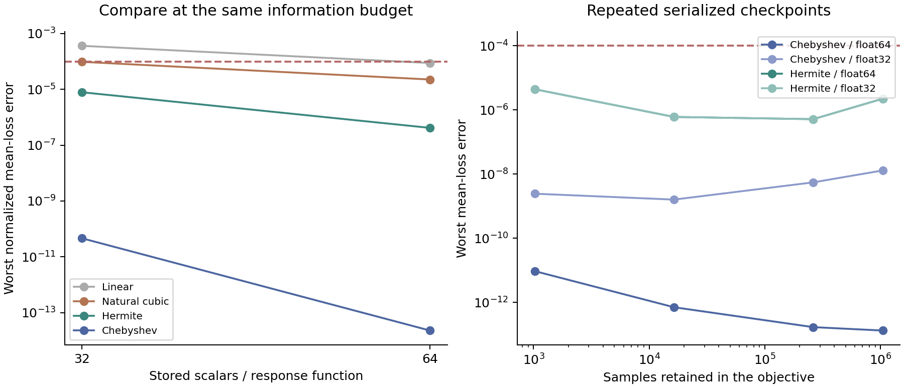
All short-panel representation budgets and long-panel storage precisions. The strong Chebyshev comparator is included. Errors concern the same declared objective, not recovery of the waveform or accuracy of the physical model.

All four long-stream arms pass every one of their 48 prefix/record checks. At 32 scalars per function, float64 objects occupy 822 bytes and float32 objects 438 bytes. Worst terminal/mean-loss errors are 3.69 × 10⁻¹⁰/9.37 × 10⁻¹² for Chebyshev float64, 2.03 × 10⁻⁸/1.30 × 10⁻⁸ for Chebyshev float32, 1.95 × 10⁻⁵/4.42 × 10⁻⁶ for Hermite float64, and 1.96 × 10⁻⁵/4.43 × 10⁻⁶ for Hermite float32. The changed headers include length and amplitude metadata, explaining their size difference from the earlier panel.

Independent SciPy statistics agree within 1.45 × 10⁻¹⁵. Whole-process high-water memory reaches 180.6 MiB, while the first encoding case reaches 106.4 MiB; later high-water marks inherit earlier evaluation allocations. A 438-byte file is not a 438-byte running program. The stream spans about 17.5 minutes, and no extrapolation to indefinite operation is measured.

9. Discussion and reproducibility

The useful property is deferred selection within a specified computational family. The representation preserves losses against the captured targets and terminal states under declared incoming states. It does not preserve arbitrary time-local events, a new target, a new nonlinear recurrence, or the ability to add unrestricted features after data deletion. These exclusions are information limits, not implementation details.

The uniform bound exploits stable analytic dependence on one parameter and normalization by record length. A likelihood sums evidence rather than averaging it; multiplying a small mean error by a long record can invalidate posterior inference. Multidimensional parameter domains also require a different approximation budget. The subsequent physical-inference study must therefore establish its own error control rather than inherit this scalar result.

The supplement contains complete summary records, frozen protocols, algebra derivation, and hashed implementation files. A separate bounded verification checks chronological composition and fixed-node merging without rerunning model selection. The contribution is a carefully specified mergeable objective representation and its resource/error tradeoff. The experiments positively support that representation while rejecting any claim that splines dominate ordinary polynomial interpolation in this setting.

10. Application boundary and research implication

This suggests a computational memory for deferred fitting, not a universal sensor codec. The stored target and recurrence define the future questions. The strong Chebyshev result is part of the conclusion: the useful object is the response-function summary, and splines are one implementation choice. Encoding cost, query count, record length, and precision determine whether the object is worthwhile.

11. Conclusion

Stable scalar dynamics admit a compact parameter-dependent record that can be queried and merged after raw samples are discarded. Fixed-node and first-jet algebra prevent additional real-arithmetic interpolation error from merge order; bounded analytic dynamics give a record-length-independent mean-loss approximation bound. Both Hermite and Chebyshev summaries work at small actual byte budgets, with Chebyshev substantially more accurate. The result is restricted computational memory, not general-purpose compression or unrestricted learning from deleted data.

References

J. H. Huggins, R. P. Adams, and T. Broderick. PASS-GLM: Polynomial Approximate Sufficient Statistics for Scalable Bayesian GLM Inference. NeurIPS, 2017. Source
L. N. Trefethen. Approximation Theory and Approximation Practice. SIAM, 2013. Chapter 8, Theorem 8.2. Source
C. de Boor. A Practical Guide to Splines. Revised edition. Springer, 2001. Source