Research manuscript · revised scientific draft
Deferred Gaussian Time-Series Inference from Lag Summaries with Record-Specific Error Bounds
Daniel Schmitter
Abstract
We investigate whether a compact measurement record can support later physical-parameter and calibration queries after its interior observations have been discarded. For a regularly sampled stationary noisy oscillator, lag products, boundaries, and a sum determine a finite-conditioning Gaussian likelihood. We combine a cancellation-free Riccati forgetting bound with retained record energy to bound its log-likelihood error for the realized record, then convert the range of likelihood errors into a posterior total-variation bound on a declared finite hypothesis grid. In 48 synthetic records and two calibrations, a 12.6 kB summary agrees with compiled exact Kalman inference to maximum posterior total variation 1.71 × 10⁻⁸ and is at least 40 times smaller than tested lossless raw storage on longer records. A separate numerical-enclosure audit passes 96 cases but costs approximately 66 minutes. Streaming capture uses 144,016 bytes of native state; all million-sample cases pass the answer-error budget, whereas six of eight four-million-sample cases fail. The study establishes a bounded deferred-inference capability and an explicit duration boundary, not continuous-posterior accuracy, real-instrument utility, or a general fixed-size memory theorem.
1. Introduction
Scientific reanalysis often changes the model or calibration rather than the measurements. A device that retains only a fitted parameter cannot support that revision. Retaining every observation permits broad reanalysis but may be costly to store or transmit. We study a middle ground: retain enough quadratic information for a declared family of stationary Gaussian calculations, together with a bound on how deleting distant conditioning information changes their answers.
The principal contribution is the specialization of Gaussian conditional factorization, Riccati forgetting, and posterior perturbation to a computable bound using only a small retained record. We provide the assumptions and derivation explicitly and test both ordinary inference and a separate arithmetic-enclosure implementation. The latter distinction is essential: observed agreement with a full-data reference is not a certificate available after those data have been discarded.
2. Related work
Vecchia approximations replace full conditioning sets with smaller selected sets [1]. State-space and semiseparable methods already make exact inference practical for relevant exponential and oscillatory covariance families; celerite is an important example [2]. We therefore compare against compiled Kalman evaluation, not an unnecessarily dense cubic-cost Gaussian solver. Fixed-size lag-based time-series estimation is also prior art, including recent VARMA work [3]. Our record-specific enclosure is a different output requirement, not a claim to have invented lag summaries.
Posterior sensitivity to likelihood perturbations has standard mathematical bounds [4]. We derive the half-L1 total-variation version used below so that its normalization and finite-grid scope are explicit. Controlled floating-point reduction and interval arithmetic are established numerical tools. Combining them with retained lag data is an engineering and analysis contribution; a passing prototype does not establish optimal compression rate or priority for the general idea of posterior-preserving compression.
3. Architecture and information flow
The capture process does not commit to one frequency, damping, gain, or offset. It retains lag products and the boundary terms needed to evaluate a finite-conditioning likelihood later. The query stage constructs its model-specific predictor from a supplied hypothesis. A separate assurance stage bounds the missing long conditioning using model contraction and energy of the retained record. These stages have different costs and must not share one latency headline.
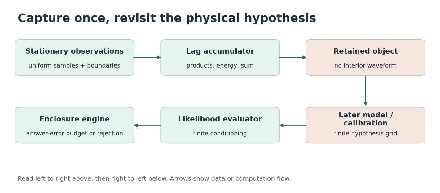
The retained energy makes the bound record-specific: a small model-average discrepancy is not automatically a small log-likelihood discrepancy for this observed record. Normalization over hypotheses then turns the range of likelihood errors into a posterior bound. The finite grid and specified noise model are part of the assertion. Agreement at grid points does not resolve a continuous posterior or identify separately confounded gain and forcing amplitude.
4. Observation model and retained statistics
The stationary latent state contains position and velocity. Frequency and damping are positive. The exact sampled model uses a matrix exponential and a process covariance chosen to preserve the stated stationary covariance. Observation noise is independent, temporally white, and added after detector gain.
The stationary position variance is fixed to one. For continuous white-noise forcing of amplitude sigma, this normalization imposes sigma squared equal to four times damping times frequency squared. It is therefore not a fixed-temperature calibration model by default. If gain and forcing amplitude were both unknown, their product would be identifiable from this channel but not both factors separately. The tested calibration changes are specified hypotheses, not a solution to that identifiability problem.
For any later covariance hypothesis, its lags determine the linear predictor from the preceding L observations and the innovation variance. The first L observations receive their exact joint Gaussian likelihood; later terms condition on the immediately preceding L samples. Expanding those residual squares gives lag products with corrections from the retained boundaries. Offset changes use the total sum and boundary terms. Thus the summary evaluates this finite-conditioning likelihood exactly in real arithmetic without retaining interior samples.
This construction does not assert that noisy oscillator observations are an order-L Markov process. Denote their exact density by p and the normalized finite-conditioning density by q. Both have the same mean. The approximation lies in the conditioning set, not in the algebra used to evaluate its chosen objective.
5. A cancellation-free model bound
Let be the stabilizing prediction-covariance Riccati solution, bounded above by the stationary state covariance S. Write H for the observation row, including gain, for the steady innovation variance, and for the closed-loop prediction matrix.
Proposition 1. The Gaussian divergence from p to q is at most B. Proof. Monotonicity of the Riccati map and its positive-semidefinite increment bound imply that the finite-past covariance excess is at most to power L times (S−) times its transpose. Therefore the excess innovation variance is at most d_L. The conditional Gaussian entropy identity expresses the divergence as one half the sum of log variance ratios between the L-past predictor and each longer-past predictor. Every denominator is at least , giving B. This avoids subtracting two nearly equal floating variances, though computing the matrix bound still requires numerical care.
6. A bound for the observed record
Let K be the exact covariance and K_tilde the covariance of q. Each normalized conditional innovation of q has unit variance under p, including the exact prefix. Consequently the relative precision matrix has trace N, and the determinant difference is twice the Gaussian divergence. If its eigenvalues are lambd, nonnegativity of each lambd−1−log(lambd) bounds every deviation from one.
Since measurement noise gives K at least RI in positive-semidefinite order, the exact whitened energy is at most E_b/R. Combining this fact with the determinant term gives the record-specific enclosure. It holds algebraically for every real record under the stated likelihood definitions, even if the physical model is misspecified.
For completeness, the eigenvalue bound follows from t−log(1+t) at least t squared divided by 2(1+t) for nonnegative t, and −t−log(1−t) at least t squared divided by two for t between zero and one. Each divergence summand is at most 2B. Solving these inequalities yields the displayed conservative delta. All quantities depending on observations are in the retained summary.
Let the likelihood-error intervals across the declared hypotheses have total range width Omega. For any common proper prior on those hypotheses, normalized posteriors satisfy the following half-L1 total-variation bound.
One derivation bounds the unnormalized likelihood ratio between positive endpoints a and b with b/a at most exp(Omega). Among bounded random ratios with a fixed mean, the absolute-deviation expectation is maximized by endpoint mass. Optimizing that mean gives (square root of b minus square root of a) divided by their sum, which is the displayed hyperbolic tangent. The same bound controls every event-probability change. A finite-grid maximum does not bound hypotheses between grid points.
Under a uniform geometric bound on powers of , B decreases like N times a geometric factor squared in L. With record energy proportional to N, this particular pathwise likelihood bound has small-B order N to the three-halves times a geometric factor in L. A lag increasing logarithmically with N and inverse tolerance is sufficient under fixed constants. This is not a lower bound or a fixed-L indefinite-duration guarantee.
7. Experimental methods
The first confirmation panel uses twelve independent seed identities, 150941–150952, two sampling intervals 0.01 and 0.05, and paired lengths 4096 and 65,536. Lengths are prefixes, not independent replications; the intervals use separate child random streams. Generating frequency is 3.1, damping 0.43, gain 1.05, and offset 0.1, with a stationary initial state. The summary fixes L=512 before evaluation.
Queries use 41 uniformly spaced frequencies from two to four and 31 dampings from 0.2 to 0.8, giving 1271 discrete hypotheses. Calibration pairs are (gain 0.9, offset zero) and (gain 1.05, offset 0.1). Uniform and fixed biased priors are both reported. The biased weights are proportional to a Gaussian in frequency centered at 2.6 with scale 0.35 and damping centered at 0.65 with scale 0.15. The true damping is not on the query grid.
Comparators are compiled exact Kalman replay, raw replay of the identical finite-conditioning likelihood, zlib-compressed raw storage, and ordinary Chebyshev banks with eight or sixteen nodes in each of frequency, damping, and gain. Bank gain ranges from 0.7 to 1.4 and offset dependence is handled analytically. Combined accuracy requires log-error oscillation at most 0.04 and posterior TV at most 0.01 under both priors. No lag or degree is selected from confirmation outcomes.
A separate arithmetic audit uses controlled pairwise binary64 products and sums with retained rounding radii. Model calculations use 80-decimal-digit interval arithmetic, verified Riccati sub/supersolutions, Toeplitz residual bounds, and enclosed prefix terms. Exact-integer operations on binary64 inputs independently verify captured statistics. The implementation relies on compiler and IEEE assumptions and on mpmath interval operations [5]; it is not a proof-assistant-verified program.
A subsequent fixed-configuration streaming panel uses two fresh seeds, both sampling intervals, and paired prefixes of 1,048,576 and 4,194,304 samples. A ring buffer and 32-level balanced-sum counter consume blocks of at most 4096 samples. The declared counter domain is N below two to the thirty-first power. Exact small-state floating references run during capture, and no raw record is retained. The same grid, lag, calibrations, priors, and TV tolerance remain unchanged.
8. Results
| Representation | Passes | Serialized bytes | Maximum posterior TV |
|---|---|---|---|
| Lag summary | 96/96 | 12,584–12,587 | 1.71 × 10⁻⁸ |
| Bank 8 | 0/96 | 16,695–16,696 | 0.1720 |
| Bank 16 | 96/96 | 131,384–131,385 | 4.86 × 10⁻⁵ |
The lag summary’s maximum likelihood-error oscillation is 1.41 × 10⁻⁷. Its normalized discrepancy from raw replay of the same finite-conditioning likelihood is 2.95 × 10⁻¹³. On longer records it is at least 40.03 times smaller than measured lossless raw storage. End-to-end capture plus two query grids takes 1.26–1.32 seconds, versus 2.00–2.08 for raw replay and 3.37–3.43 for the accurate bank. On shorter records the summary takes 1.27–1.29 seconds while raw replay takes only 0.126–0.127 seconds. The accurate bank also has faster warm queries.
The arithmetic-enclosure audit passes all 96 cases with maximum posterior-TV bound 0.0002971 and retained size 12,695–12,700 bytes. All 24,624 audited lag statistics enclose their exact-integer values. All 122,016 full-record floating likelihood references are contained. The query phase takes 3954.83 seconds, approximately 66 minutes, and verification 56.05 seconds. This assurance cost must not be conflated with the ordinary second-scale inference timings.
| Samples | Interval | Bound passes | Maximum TV bound |
|---|---|---|---|
| 1,048,576 | 0.01 | 4/4 | 0.004442 |
| 1,048,576 | 0.05 | 4/4 | 0.003047 |
| 4,194,304 | 0.01 | 0/4 | 0.018431 |
| 4,194,304 | 0.05 | 2/4 | 0.012205 |
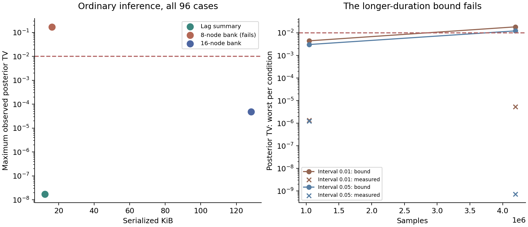
Native accumulator storage is 144,016 bytes and retained objects occupy 12,700–12,703 bytes. All resource criteria pass. All million-sample cases satisfy the answer bound, but six of eight four-million-sample cases fail, so the complete scale-up criterion fails. All 20,336 floating likelihood references remain inside their intervals; maximum observed posterior TV is 5.37 × 10⁻⁶. Small observed error does not override rejection by the prescribed computable bound.
Counting each of four streams only once through its longest prefix, candidate append work takes 6.127 seconds, compared with 485.206 seconds for the simultaneously accumulated reference workload. The latter is not an optimized minimal answer bank. Enclosed querying takes 2909.88 seconds, with substantial shared model preparation. Capture peak RSS is 117.2 MiB. The coarse grid has effective posterior support only 1.0–1.854 points, precluding a resolved continuous-uncertainty claim.
9. Discussion and reproducibility
A smaller exact control exists when every later query is predetermined: storing one binary64 likelihood per grid point for both calibrations needs 20,336 payload bytes before metadata. That calculation moves the work into capture and cannot support unlisted queries. The present summary’s value lies in parameter-independent capture and deferred model calculations, not in a false comparison where every alternative must retain the waveform.
Finite marginal dependence must not be confused with finite conditional memory. For Gaussian increments with lag covariances 2/3, 1/6, and zero, the conditional covariance at distance two given the middle variable is −1/24. Compactly supported innovation kernels therefore do not justify discarding conditioning error. The present likelihood deliberately includes that approximation and its bound.
The supplementary record contains the frozen protocols, complete aggregate outcomes, derivation, source fingerprints, and integrity reports. Independent reference containment is a strong numerical check but not a formal solver proof. Uniform sampling, stationarity, known post-gain noise, specified calibration hypotheses, and a finite grid are substantive restrictions. No hardware energy result, arbitrary gap handling, or real optical-trap or machinery decision is established.
10. Application boundary and research implication
This is a candidate instrument-memory interface with a refusal condition. Longer duration can exhaust a fixed lag budget even while observed numerical error remains small. Reporting that refusal is more useful than silently weakening the error target. A real instrument would additionally need qualified gaps, drift, calibration uncertainty, and a useful downstream inference decision.
11. Conclusion
Lag summaries can retain enough information to revise a stationary Gaussian interpretation after interior data are discarded. A record-energy bound converts model forgetting into a posterior error budget computed from the retained object. The tested implementation provides accurate compact inference and passes a separate numerical audit, while exposing expensive assurance, short-record disadvantages, and a failed longer-duration boundary. The result is an auditable restricted reanalysis primitive, not universal lossless scientific memory.
References
- M. Katzfuss and J. Guinness. A General Framework for Vecchia Approximations of Gaussian Processes. Statistical Science 36(1), 124–141, 2021. Source
- D. Foreman-Mackey, E. Agol, S. Ambikasaran, and R. Angus. Fast and Scalable Gaussian Process Modeling with Applications to Astronomical Time Series. Astronomical Journal, 2017. Source
- D. Paulin and V. Elvira. Scalable Estimation of VARMA Models. arXiv:2608.06340, 2026. Source
- A. Doucet. A Note on the Sensitivity of the Posterior Distribution to the Likelihood Function. Author technical note. Source
- mpmath developers. Arbitrary-Precision Interval Arithmetic. Official documentation; interval context limitations. Source