Research manuscript · revised scientific draft

Exact Operator Cells for Compact Option-Pricing Services: Stability, Workload, and Single-Thread Deployment

Daniel Schmitter

Abstract

Operator-matched local solutions can eliminate spatial interior unknowns before repeated pricing calculations. We describe a layered one-dimensional European diffusion implementation using exact cell boundary maps, structured inverse readouts, and stable confluent source propagation. Two archived studies quantify distinct benefits. Selective treatment of nearly coincident poles reduces complete three-interval calculation time from 63–117 ms to 4–12 ms on twelve exposed synthetic cases, while failing a separate artifact-storage budget. A native single-thread application returns 23 enclosed prices and two finite spot responses with 4.793 ms warm median latency and 2.219 MiB peak process memory on an Apple M4 Max. A matched residual-certified polynomial comparator qualifies six of twelve cases at its largest tested mesh; only those joint qualifications support relative-cost claims. These results establish bounded computational capabilities, not a general pricing-theory advance, low-power-device result, market calibration success, or executable profitability. The contribution is a reproducible integration of operator elimination, conditioning-aware representation, and complete serving-cost measurement.

1. Introduction

A real-time model service must pay for more than its final function evaluation. It may rebuild a coefficient field, assemble a numerical operator, answer a batch of contracts, and serialize outputs. A compact representation can help when those reconstruction costs dominate, even if an ordinary polynomial interpolant answers prepared queries faster. This workload distinction motivates the present study.

We consider supplied European diffusion models, not prediction of future returns or the discovery of tradable prices. The contribution is an engineering and numerical study: exact local elimination, stable representation across operator changes, and measured native deployment. The experiments separate ordinary point evaluation from numerically enclosed outputs and retain unsuccessful comparators and resource gates.

2. Related work and model

Analytic spatial solutions after a Laplace transform have close local-volatility prior art, including the Lipton–Sepp construction and its extension by Itkin and Lipton [1]. Rational time inversion is established numerical analysis [2]. Inner-product calculus motivates evaluating continuous products through basis coefficients [3], but periodic cardinal identities cannot be transplanted into a bounded heterogeneous pricing operator. Our financial cells are nonuniform and coefficient-dependent, not a single cardinal B-spline basis.

For a normalized positive martingale X with local volatility sigma(log X), set a equal to sigma squared divided by two. The backward generator in logarithmic state is a(x)(D squared minus D). On a bounded interval, subtracting the payoff and conjugating by an exponential gives the time-value resolvent

\left[-D_x^2+\frac14+\frac{s}{a(x)}\right]\widehat w(s,x;y)=\frac{e^{y/2}}s\delta_y,\qquad C(t,e^x;e^y)=(e^x-e^y)_++e^{x/2}w(t,x;y).

The payoff-subtracted time value has homogeneous Dirichlet boundaries, corresponding to stopping and holding the asset at the domain endpoints. A deterministic discount is applied under each archived contract. The coefficient field and reference coordinate remain fixed during spot perturbations. A stationary field in a drift-normalized coordinate is not automatically stationary in physical spot when carry is nonzero.

3. Architecture and information flow

The numerical service has a preparation stage and an output stage. For each time-inversion parameter, local differential equations produce two-endpoint cell maps. Interface matching gives a structured solve; selected readouts reuse that solve across output requests. Changing maturity slabs requires carrying an inhomogeneous source representation, not only endpoint values. Near pole collisions, that representation remains in a confluent form to avoid cancellation.

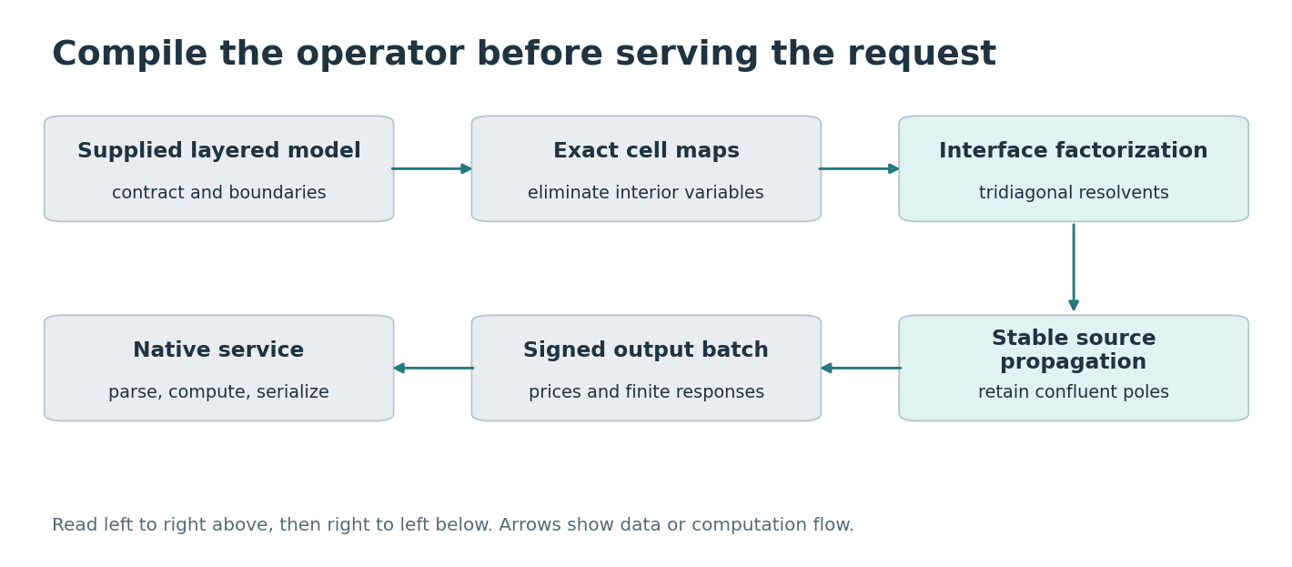
Compile the operator before serving the request. Boxes distinguish supplied information, fitted components, and the quantity evaluated. Arrows show computation or data dependence, not a newly trained deep network.

This is an operator compiler rather than a trained pricing network. Its small state follows from exact elimination for the declared layered model, not from discovering a universal low-dimensional option surface. The output workload determines the relevant alternative: a prefactored solve can win for one contract, a prepared polynomial can win for warm queries, and exact cells can win when a model is rebuilt and many quantities are enclosed together.

4. Exact cell elimination and readouts

On a cell of width h with constant q equal to one quarter plus s/a, let the pole p be a square root of q. Endpoint values determine the homogeneous interior through hyperbolic basis functions. Their outward derivatives are obtained from a two-by-two boundary matrix:

H_L(x)=\frac{\sinh(p(h-x))}{\sinh(ph)},\quad H_R(x)=\frac{\sinh(px)}{\sinh(ph)},\qquad N(q)=\begin{pmatrix}p\coth(ph)&-p\operatorname{csch}(ph)\\-p\operatorname{csch}(ph)&p\coth(ph)\end{pmatrix}.

Matching fluxes assembles a complex-symmetric tridiagonal system on native interfaces. Local payoff sources contribute endpoint loads plus an inhomogeneous cell correction. This elimination is exact for the declared piecewise-constant spatial equation, not for an arbitrary smooth volatility field approximated by it. Stable elementary formulas handle small cells and decaying exponentials. Complex symmetry is bilinear, not Hermitian.

At a fixed observation point, many strikes can reuse selected rows of the inverse after factorization. Conversely, a single strike may be cheaper with an ordinary prefactored solve. A coefficient change in one cell changes only its two-endpoint block, allowing classical finite-rank updates. Neither selected inversion nor finite-rank algebra is unique to splines; whether it helps depends on the output batch and preparation cost.

5. Changing operators and confluent source state

A later maturity interval is forced by the preceding curve, which is generally inhomogeneous within each cell. Retaining only its endpoint values is therefore insufficient. Green’s identity supplies cross-operator basis products from boundary-map divided differences, with a derivative limit when the parameters coincide:

\int_0^h H(q,x)H(r,x)^T\,dx=\frac{N(q)-N(r)}{q-r},\qquad r\to q:\quad\int_0^hH(q,x)H(q,x)^T\,dx=N'(q).

The ordering convention identifies H as the two endpoint basis functions; the identity is bilinear at complex parameters. Expanding a forced response into distinct pole terms can create enormous opposing coefficients near a collision. Retaining its divided-difference form avoids that expansion, and a repeated pole becomes a parameter derivative. This is the same confluent principle that connects repeated roots with polynomial-exponential or Hermite forms.

The measured implementation retains close pairs in a stable confluent form and expands only separated pairs. The relative squared-pole threshold 0.05 was fixed before the comparison. The compiled source owns its arrays, removing repeated evaluation of the full preceding object. This is selective algebraic evaluation, not lossy fitting or a proof of cheap closure across arbitrarily many maturity intervals.

6. Experimental methods

The selective-confluence study reuses 34 source cases and twelve three-interval cases, including four constant controls and eight layered fields. Both methods use the same 24-node contour, 32-point source quadrature, nine strike readouts, and independent qualified references. Seven complete cold constructions per method and case use rotated order. Price, strike-slope and density are distinct outputs; they are not spot Greeks. All cases were previously exposed, and no threshold search is performed.

The deployment study instead returns 23 price intervals and two signed spread finite responses from a supplied maturity and fifteen log-volatility parameters. Twelve exposed cases comprise six fields and two maturities. The exact and polynomial implementations share the bounded-domain model, 24-node time inversion, interval arithmetic, sources and readouts. Qualification requires containing the independent reference intervals and widths at most 2 × 10⁻⁸ for prices and 4 × 10⁻⁸ for responses.

The polynomial comparator uses consistent-mass linear finite elements, cubic primal–dual residual correction, focused sinh meshes, interface/readout preservation, and midpoint subdivision. Four fixed base budgets are tested. Both paths perform native construction. One warm-up, three warm repetitions, and one new-process request per case are retained; method order is fixed. Request latency includes parsing, calculation, serialization and pipe transport. Cold startup does not flush the operating-system page cache. One worker and one observed computation thread are used on a shared Apple M4 Max, without core affinity or controlled host load.

7. Results

Native enclosed-output comparison. Latency includes all cases; it is not an accuracy-matched speed ratio.
Method	Qualified cases	Warm median (ms)	Peak RSS (MiB)
Exact cells	12 / 12	4.793	2.219
Polynomial 32	0 / 12	29.112	2.344
Polynomial 128	0 / 12	69.931	2.516
Polynomial 512	1 / 12	244.119	3.844
Polynomial 2048	6 / 12	926.699	8.406

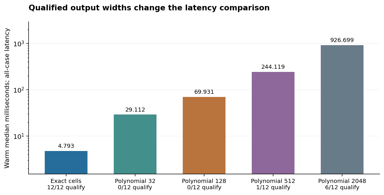
All-case native warm median latency with numerical qualification counts. Unqualified cases cannot supply matched-accuracy speed ratios. The paper reports ratios only where both implementations qualify.

All comparator intervals contain the references; failed qualifications are intervals that remain too wide. On the six jointly qualifying cases, the smallest tested qualifying polynomial budget costs 52.75–206.04 times the exact method. This is a descriptive frontier on exposed cases, not a frozen adaptive selection rule or a comparison against optimized high-order finite elements. The remaining six cases have no assigned speed ratio.

The exact application’s warm p95 is 5.045 ms and launch-inclusive cold p95 is 8.718 ms. Its executable is 139,064 bytes and uses system C++ libraries, with no Python, BLAS, GPU or thread pool at runtime. The separate benchmark driver peaks at about 36.25 MiB. Native process memory must not be confused with total development or harness memory. All ten predeclared calculator/recipient application gates pass; recipient verification is detailed in the companion certificate study.

Selective confluence passes every source and pricing accuracy check. Complete three-interval time is 4.09–12.28 ms versus 63.30–117.35 ms, a paired internal gain of 5.30–17.18. However, retained study artifacts total 132,999 bytes against a 102,400-byte budget. The driver stops after saving the results and before final RSS/elapsed capture. That missing resource record is not reconstructed from another run, and the study is not described as passing all gates.

Earlier unverified prepared-query comparisons expose the workload boundary: an ordinary prepared polynomial curve answers 501 queries faster, while exact cells reduce reconstruction-plus-query cost and retained arrays. Likewise, selected inverse rows lose most one-contract comparisons. Finally, layered coefficients can make left and right spot curvatures differ at an interface. The earlier right-trace accuracy check did not establish a unique classical gamma. The current native interface returns finite responses, not a smooth-gamma hedge guarantee.

8. Discussion

The measured result is a small native numerical service on a powerful workstation. It supports the feasibility of modest-runtime implementations but does not measure weaker hardware, energy, hard real-time latency, or financial usefulness. A failed market-admission campaign remains failed despite these timings. Conventional adaptive methods and established financial libraries have not been exhausted.

The operator toolbox contributes most clearly when it removes spatial approximation work, preserves signed calculations, and avoids ill-conditioned coordinate expansions. The strongest transferable result is a disciplined separation of representation, numerical guarantee, preparation cost, and serving cost. The supplement retains source hashes, protocols, aggregate results, and all failed qualifications rather than selecting only the headline timing.

9. Application boundary and research implication

A practical service must include request parsing, construction, arithmetic guards, output formatting, and process memory. The one-thread measurements do so for the named requests on the local workstation. They do not establish a weaker-device result or financial utility. The market-admission failure remains a separate, unresolved application boundary.

10. Conclusion

Exact operator cells and conditioning-aware source compilation yield useful, bounded implementations for supplied layered European models. The single-thread application meets its declared numerical and resource gates; selective confluence removes a measured internal bottleneck while failing a separate storage gate. These are reproducible computational results, not evidence that market inference or general option pricing has been solved.

References

A. Itkin and A. Lipton. Filling the gaps smoothly. Journal of Computational Science, 2018; author preprint, 2016. Source
L. N. Trefethen, J. A. C. Weideman, and T. Schmelzer. Talbot Quadratures and Rational Approximations. BIT 46, 653–670, 2006. Source
A. Badoual, D. Schmitter, and M. Unser. An Inner-Product Calculus for Periodic Functions and Curves. IEEE Signal Processing Letters 23(6), 878–882, 2016. Source