Research manuscript · revised scientific draft
Price Agreement Does Not Identify Local Risk: Thin-Layer Limits and a Bounded Market-Admission Study
Daniel Schmitter
Abstract
Accurate option prices do not necessarily identify point curvature. We give a bounded-domain thin-layer construction in which prices converge to those of a constant diffusion while at-the-money point gamma retains an inverse local-coefficient factor. Fixed nonzero bump responses instead converge to the background response, so the small-layer and small-bump limits do not commute. A finite noisy quote panel consequently cannot uniformly identify point gamma over this unrestricted thin-layer family. We then distinguish this analytical result from constructive synthetic ambiguity witnesses and from a completed real-data admission failure. In five public-feed capture episodes, all 92 saved model proposals fail the prescribed conservative quote-compatibility procedure; the 120 planned risk directions are therefore not tested. The numerical operator remains accurate on saved-field comparisons, but no market-risk application is established. The contribution is an output-specific identifiability analysis and a transparent account of the gap between numerical capability and model admission, not a trading strategy or general market impossibility theorem.
1. Introduction
A pricing solver answers a conditional question: what follows if this model is supplied? Calibration asks which supplied models observations permit. A risk output may be much more sensitive to the distinction than the fitted prices. Faster or more accurate arithmetic does not remove that inverse problem.
This paper gives a concrete analytical example and connects it to two separate evidence levels. Synthetic verified pairs demonstrate the existence of materially different compatible finite responses under a declared observation model. A later public-market study fails before that test because no candidate is admitted. These outcomes are related scientifically but must not be pooled as repeated demonstrations of market usefulness.
2. Related work
Local-volatility calibration and its regularization are established inverse problems [1]. Analytic transformed local-volatility models provide the spatial tools used here [2]. The thin-layer argument specializes ordinary Green and spectral analysis; it is not a claim of first discovery of instability in calibration. The settlement adapter used in the market study applies classical conditional Jensen and convex-order reasoning, with substantial Asian-option bounding prior art [3].
3. Architecture and information flow
The market pipeline must define the observed contract before fitting an operator. A terminal-payoff model and an averaged-settlement quote are not the same object. The adapter supplies an enclosure under stated martingale assumptions, and admission requires its complete containment in each quote band. Only admitted candidates would advance to risk comparisons. In the completed campaign none did, so the risk directions remain untested rather than negative risk estimates.
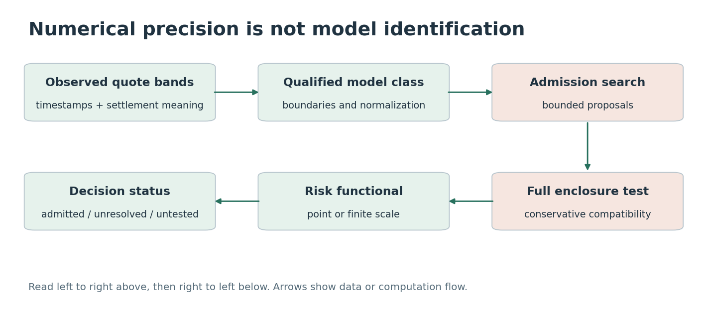
The thin-layer analysis is a separate information result. Price observations smooth over a shrinking region while point curvature retains sensitivity to its local coefficient. A fixed finite bump asks a different spatial-scale question. The noncommuting limits explain why greater arithmetic accuracy does not resolve the inferential ambiguity and why a risk specification must include its perturbation scale.
4. A thin-layer construction
Fix a finite log domain minus L to L and strictly positive constants and , independent of epsilon. Let equal inside the open interval of radius epsilon around zero and elsewhere. The asset satisfies dZ equal times Z dW, stopped and held at the two domain boundaries. Let be the expected call payoff at fixed positive maturity. The background uses everywhere.
Proposition 1. At each fixed positive maturity, prices at fixed interior strikes or starting states converge to the background prices as epsilon tends to zero. At spot and strike one, classical point gamma instead tends to / times the background gamma. For any fixed positive bump h with both bumped states interior, central finite-bump gamma converges to its background value.
The point gamma exists for every positive epsilon because the spot lies strictly inside a constant-coefficient neighborhood. This is not a one-sided interface trace or a coefficient changed only at one isolated point. The proposition excludes maturity shrinking with epsilon, coefficients approaching zero or infinity, and an unbounded-domain limit.
5. Proof through positive real resolvents
Subtract the payoff , defined as the positive part of exp(x) minus exp(y), conjugate by exp(minus x/2), and take the Laplace transform. With x equal to log z and y equal to log k, the transformed time value satisfies the operator equation below. Its Green kernel uses ordinary coordinate measure, not the weighted spectral measure.
For real positive s, set to , to , and propagate the right logarithmic derivative across the central half-layer. Symmetry gives
For fixed nonzero y outside the shrinking layer, matching multiplies this diagonal value by the reciprocal of , and by . These factors converge to the background factors. Green symmetry gives the corresponding fixed-start result.
We use a monotone Laplace-continuity lemma to pass to fixed time, rather than differentiating a pointwise price limit. If nonnegative functions are all monotone in the same direction, their finite Laplace transforms converge at every positive argument to that of a continuous limit, then their values converge at every positive time. To see this, exponentially weight the functions into finite measures and map time to exp(minus time) on the compact unit interval. Convergence of all integer moments and polynomial density gives weak convergence. Integrals over neighboring time intervals then squeeze the monotone function values; shrinking the intervals yields the continuous limit.
Stopped assets are bounded martingales, so convex call expectations are nonnegative and nondecreasing in maturity. The lemma therefore proves the price convergence. For the time derivative at the diagonal, use the positive weighted Sturm–Liouville expansion [4] with weight 1/. Its diagonal heat series is a sum of squared eigenfunction values times exp(minus eigenvalue times time), hence nonnegative and nonincreasing. Its Laplace transform is the diagonal Green kernel. The resolvent bounds its derivatives on every time interval bounded away from zero, so the background series is continuous and the same lemma applies.
At the center, that heat series equals the call’s maturity derivative. The backward equation gives equal to , while the background gives equal to . Dividing the convergent heat series proves the gamma factor. The fixed-bump conclusion follows from the three already-convergent prices. Interior regularity at each fixed epsilon and then at the background proves the distinct iterated limits:
6. Information consequence
For any finite set of fixed interior strikes and positive maturities, the quote mean vectors converge. With fixed strictly positive independent Gaussian noise scales, their whitened distance tends to zero, and optimal equal-prior discrimination error tends to one half. Yet the gamma values remain separated when differs from . An estimator accurate to less than half that separation would distinguish the two models by the closer gamma, so its average failure probability is at least the optimal testing error. Uniformly reliable point-gamma recovery is therefore impossible over this family with these observations.
This conclusion does not cover a common minimum layer width, vanishing quote noise, very short maturities resolving the layer, path observations, or additional physical assumptions. Nor does convergence of fixed-bump risk prove its identification from an arbitrary sparse surface. It shows why the risk quantity and its spatial scale must be part of the question.
7. Experimental methods
The associated synthetic thin-layer study uses background volatility 0.20 and central volatility 0.10 or 0.40, predicting limiting gamma ratios four and one quarter. Its explicit resolvent is checked against the independent exact-cell assembly. These finite checks validate signs and matching; the proof above, not a finite sweep, supplies the limiting claim. Separate shared-surface witness experiments use finite spot responses and cannot be substituted for this point-gamma theorem.
The external study freezes a cohort of 102 public Deribit linear BTC_USDC option instruments: seventeen paired call/put strikes at each of three expiries. Five capture episodes, including development and four prospective slots, produce twenty overlapping views. Those views are correlated, not twenty independent sessions. Exercise, normalization, timestamps, quote uncertainty, and the thirty-minute averaged settlement are explicitly qualified. Raw vendor records are not redistributed because their redistribution rights are unresolved.
For a deterministic forward normalization and a positive true martingale X, conditional and pathwise Jensen sandwich a convex average-payoff expectation between terminal expectations at the averaging start and end. The adapter widens both endpoints by numerical error. The sufficient admission rule requires the entire resulting price enclosure to lie inside each quote band, not merely intersect it. Failure of this conservative rule does not prove the model’s actual average price is incompatible. A later scalar-clock variant retains the same spatial generator and changes deterministic elapsed variance; it is not a general time-dependent volatility surface.
8. Results
| Episode UTC | Views | Final slack range | Admitted |
|---|---|---|---|
| Development | 4 | 0.980–1.514 | 0 |
| 07:00 | 4 | 1.390–1.672 | 0 |
| 10:00 | 4 | 1.909–2.436 | 0 |
| 13:00 | 4 | 0.937–1.825 | 0 |
| 15:00 | 4 | 3.183–4.274 | 0 |
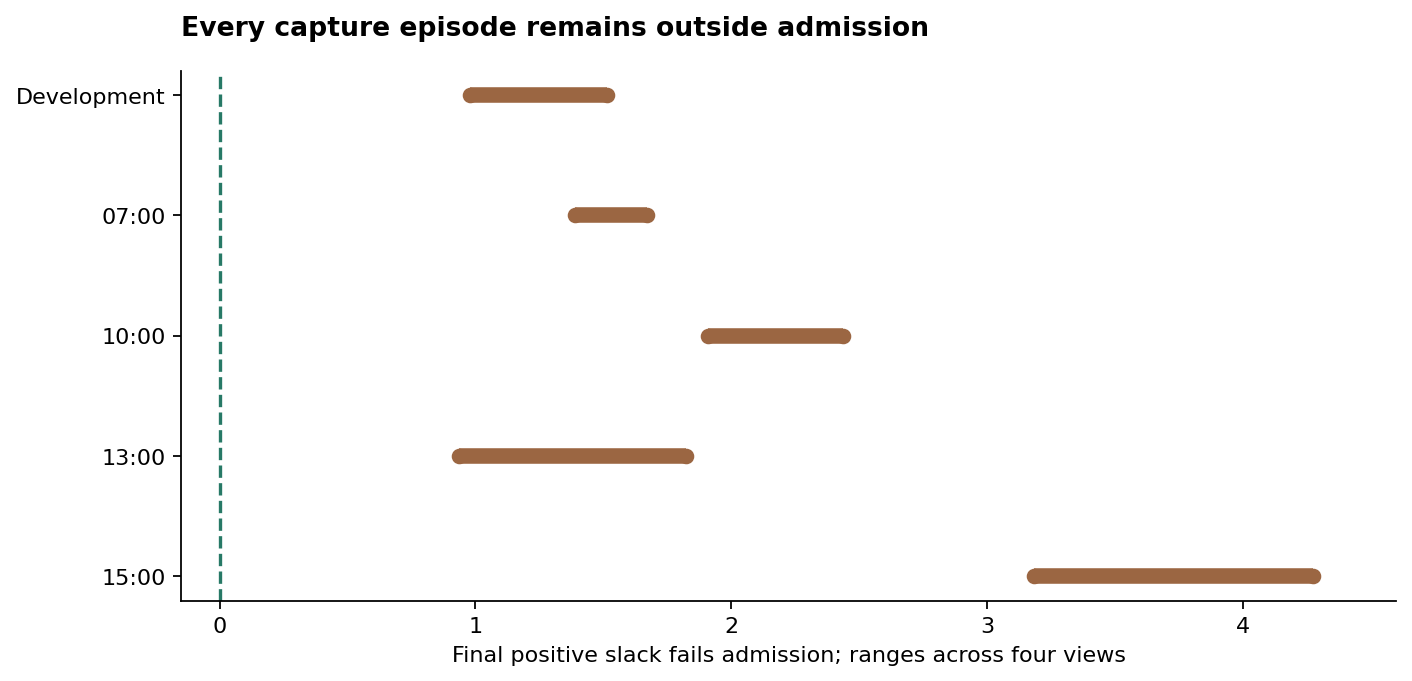
Across the bounded campaign, twelve homogeneous proposals, sixty clock-study midpoint proposals, and twenty direct-feasibility proposals fail the prescribed admission. All 120 planned risk directions are explicitly untested. Optimizer success is not admission: fifteen of the twenty direct searches report numerical success, yet every final point misses quote bands. A subsequent exact-rational necessary-band check finds no elementary within-expiry contradiction in sixty blocks; it does not establish joint model feasibility or identify the source of failure.
The numerical component remains capable. On 120 saved-field terminal reference cases it uses 38 spatial nodes and 3,872 persistent-array bytes, taking 0.602–1.389 ms with maximum error bounds below 4.69 × 10⁻¹². The finest prescribed finite-element meshes use approximately 4,816 nodes and take 5.000–8.322 ms, with larger errors. These are not accuracy-matched speed ratios, optimized finite-element benchmarks, or whole-process memory comparisons. Forty final unit tests and replay of all 92 proposal prechecks pass without rerunning optimization.
9. Discussion
The theorem, synthetic witnesses, and external failure have different scopes. Thin layers expose a structural identifiability limit. Verified pairs establish an existential ambiguity under a supplied synthetic contract. Failed public-data admission establishes that this bounded procedure did not reach a usable market-risk test. None supports profitable trading, general infeasibility of the local-volatility class, or identification of a unique defect in the proposer.
A scientifically useful next model would first need a market-compatible observation interface and an established calibration comparator. The completed campaign is not tuned further to rescue its outcome. Original local feed files remain necessary for exact data replay; published hashes alone cannot reconstruct them. The publication supplement contains first-party protocols, derivations, aggregate accounting and source identities, not restricted quote records.
10. Application boundary and research implication
The resulting application design has two independent gates: compute the supplied model accurately, and establish that observations support the model-dependent question. Faster computation helps the first. The campaign failure prevents a claim about the second, without proving that the entire model class is infeasible or that no alternative admission method could succeed.
11. Conclusion
Point-price agreement and point-risk identification are different mathematical properties. A thin-layer family makes that distinction explicit, while a completed market study demonstrates the separate necessity of qualified model admission. Accurate, compact operator calculations remain a useful computational component, but they do not by themselves establish a market-risk application.
References
- S. Crepey. Calibration of the Local Volatility in a Generalized Black–Scholes Model Using Tikhonov Regularization. SIAM Journal on Mathematical Analysis 34(5), 1183–1206, 2003. Source
- A. Itkin and A. Lipton. Filling the gaps smoothly. Journal of Computational Science, 2018; author preprint, 2016. Source
- A. Novikov and N. Kordzakhia. On lower and upper bounds for Asian-type options: a unified approach. 2013. Source
- NIST Digital Library of Mathematical Functions. Sturm–Liouville equations and spectral expansions, Sections 1.13(viii) and 1.18(v). Source