Research manuscript · revised scientific draft

Separating Physical Constraints from Statistical Estimation in Operator-Structured Models

Daniel Schmitter

Abstract

A representation can satisfy a differential equation exactly while estimating its solution poorly. We develop a modular formulation that separates supplied linear physics, observation-based coefficient estimation, and forward prediction. For a fixed operator-compatible basis, physical feasibility is independent of fitted coefficients, whereas identifiability and noise amplification depend on the observation matrix. We derive the corresponding error and variance relations and test them in controlled Helmholtz and heat-equation examples. With 24 sensors and 5% Gaussian observation noise, a two-mode Helmholtz estimator has median relative field error 1.05% over 20 noise realizations for distributed sensors, but 88.6% for tightly clustered sensors; both estimates satisfy the same homogeneous equation. In a six-mode heat example, an estimated initial condition yields 2.09% space-time error with the correct diffusivity and 12.8% with a misspecified diffusivity. These new mechanism studies are distinguished from an archived periodic spectral-solve/PINN comparison and prior constitutive-identification results. The contribution is a reproducible account of where operator structure removes optimization and where statistical learning remains necessary, not a new spectral solver or a universal replacement for physics-informed neural networks.

1. Introduction

Scientific prediction combines knowledge that is already available with quantities that must be inferred. A differential equation may be supplied while its initial condition is unknown; a conservation law may be established while a material response must be learned. Treating all these unknowns as unconstrained neural weights can obscure this distinction. Conversely, encoding a known equation in a basis can make numerical accuracy look like scientific discovery when the basis already contains the answer.

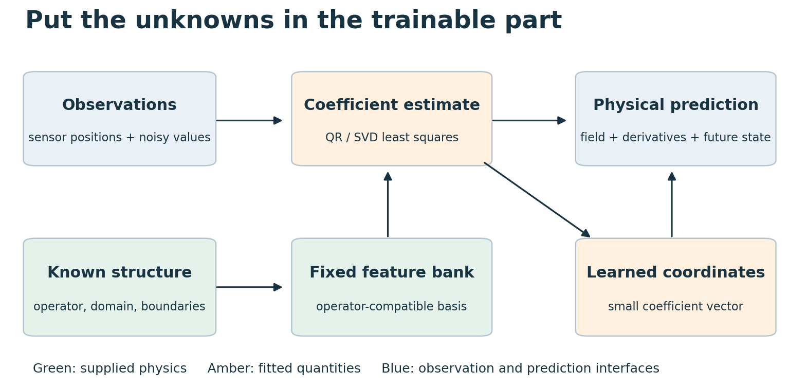
We study a decomposition into an observation interface, a fixed operator-compatible feature map, a coefficient estimator, and a synthesis or evolution module. The central question is not whether a neural network can represent a field, but which variables genuinely require optimization. Our contributions are a self-contained formulation of the decomposition, an explicit separation of physical feasibility from statistical recoverability, and controlled sensor and propagation experiments that expose both its advantages and its failure modes. The experiments are deliberately small enough for every assumption to be inspected.

Implemented module structure for the fixed-basis examples. The operator, boundaries, and basis are supplied. Sensor values determine coefficients through least squares; the fitted coefficients then drive synthesis or exact modal propagation. This is a shallow fixed-feature model, not a diagram of a trained deep neural network.

2. Related work

Physics-informed neural networks represent a solution with a neural function and incorporate differential-equation information through the training objective [1]. Hard-constraint representations and classical spectral methods provide a different allocation of known structure [2]. Exponential splines associate compactly supported generators with differential operators and reproduce exponential-polynomial functions under appropriate conditions [3]. Periodic spline inner-product calculus converts continuous objectives into coefficient-domain matrices [4]. None of these principles is introduced here.

The present work makes their interfaces explicit for learning problems: the observation operator determines what can be identified, the representation determines what can be expressed, and the physical evolution determines what can be propagated. Sparse identification of dynamics supplies a related strategy when only a constitutive component is unknown [5]. Our Fourier examples are not exponential B-spline implementations; they isolate the operator mechanism before introducing local spline parameterizations. Operator matching alone therefore cannot establish a spline-specific advantage.

3. Architecture and constrained estimation

Let a linear differential operator and homogeneous boundary conditions define an admissible space. Choose a particular solution for any known forcing and inhomogeneous boundary data, and homogeneous basis functions satisfying the remaining constraints. Let H denote the observation operator, including sensor locations or integral measurements. The model is

u_c=u_p+\Phi c,\quad \mathcal L u_p=f,\quad \mathcal L\Phi=0,\qquad y=Hu_c+\varepsilon,\quad A=H\Phi.

Boundary conditions must also be satisfied by the particular solution and homogeneous basis. A family of sine and cosine solutions of an interior equation does not automatically satisfy arbitrary boundary data. If those boundaries are unknown, they remain part of inference. With a fixed basis, unregularized coefficient estimation is linear least squares; a continuous quadratic regularizer can be added when appropriate:

\widehat c=\arg\min_c\|Ac-(y-Hu_p)\|_2^2+\lambda c^TQc,\qquad Q_{ij}=\langle D\phi_i,D\phi_j\rangle.

The experiments use unregularized least squares through an SVD-based library routine, not an explicit normal-matrix inverse. Full column rank gives uniqueness without regularization. With a positive regularizer, uniqueness instead requires that the null spaces of A and Q have trivial intersection. For local spline spaces, Q can be banded; periodic translation invariance may make it circulant. Neither structure follows for an arbitrary sensor normal matrix. Learning basis poles or sensor coordinates changes A and may reintroduce nonlinear optimization.

4. Feasibility is not recoverability

Proposition 1. Every fitted coefficient vector satisfies the encoded homogeneous equation, independently of observation noise. If the true field belongs to the supplied affine space and A has full column rank, the coefficient error is A-dagger times the observation noise. Proof: linearity gives the equation identity, and substitution of the observation model in the least-squares solution gives the error expression.

\mathcal L\widehat u=f,\qquad \widehat c-c_*=A^\dagger\varepsilon,\qquad \|\widehat u-u_*\|\le\|\Phi\|\,\|A^\dagger\|\,\|\varepsilon\|.

For independent zero-mean noise with variance sigma squared, the expected integrated squared field error is determined by the physical Gram matrix G. This is a statistical property, not a PDE residual:

G_{ij}=\langle\phi_i,\phi_j\rangle,\qquad \mathbb E\|\widehat u-u_*\|_{L^2}^2=\sigma^2\operatorname{tr}\!\left(G(A^TA)^{-1}\right).

Proposition 2. If the true field contains an unrepresented component r, then the prediction error consists of propagated observation noise and a representation-dependent bias. Writing the true field as the supplied particular solution plus a represented component and an unrepresented remainder gives

\widehat u-u_*=\Phi A^\dagger\varepsilon+(\Phi A^\dagger H-I)r.

An exact residual for the supplied operator cannot detect that the supplied operator is wrong. Nor can it show that a homogeneous basis spans all solutions allowed by the physical boundary conditions. These two propositions are standard linear estimation identities; here they explain why increasing physical exactness need not improve prediction.

5. From static reconstruction to physical evolution

For heat diffusion on the unit interval with zero endpoint temperatures, a sine basis supplies exact spatial boundary conditions and modal evolution. The unknowns are the initial amplitudes; the diffusivity is supplied.

u_t=\kappa u_{xx},\quad u(0,t)=u(1,t)=0,\qquad u(x,t)=\sum_{j=1}^{m}c_j\sin(j\pi x)e^{-\kappa(j\pi)^2t}.

Estimating the initial amplitudes and propagating them are distinct operations. Orthogonality yields a contraction of the represented initial-state error for positive diffusivity:

\|\widehat u(t)-u_*(t)\|_{L^2}^2=\tfrac12\sum_j(\widehat c_j-c_{*,j})^2e^{-2\kappa(j\pi)^2t}\le\tfrac12\|\widehat c-c_*\|_2^2.

This is forward stability, not stable recovery of an initial state from late measurements. Reversing the decay amplifies high-frequency errors. A wrong diffusivity also changes the propagator and falls outside the displayed bound. For an unknown diffusivity, coefficient estimation can be nested inside a separate parameter-estimation problem; that extension is not tested here.

The same division of labor has a connection to constant-volatility Black-Scholes pricing. With constant volatility sigma, interest rate r, and dividend yield q, the log-price and time-to-maturity coordinates give diffusion, drift, and discounting [6]:

V_\tau=aV_{xx}+bV_x-rV,\quad a=\tfrac12\sigma^2,\quad b=r-q-a,\qquad \widehat V(\omega,\tau)=e^{(-a\omega^2+i b\omega-r)\tau}\widehat V(\omega,0).

The Fourier expression assumes a setting where the transform is valid. Vanilla payoffs are not periodic and need growth handling, domain treatment, or a different transform. Local volatility, barriers, and exercise constraints change the problem. We include this derivation to show a structural connection, not a new pricing result or a claim that a two-mode heat demonstration validates an options engine.

6. From operator modes to cardinal-spline computation

The global harmonic examples explain constraint elimination, but local exponential B-splines do not individually lie in the global homogeneous null space of their generating operator. Applying that operator produces localized innovations at knots. Exponential reproduction means that appropriate coefficient combinations reproduce the desired exponential-polynomial functions; it does not mean that arbitrary local coefficients satisfy a homogeneous PDE. This distinction prevents a false extension of the two-mode example.

For a local spline expansion, a second route compiles a continuous operator-residual objective into reusable coefficient-domain matrices. With an operator Gram matrix K and forcing inner products d, finite expansion gives

K_{ij}=\langle\mathcal L\phi_i,\mathcal L\phi_j\rangle,\quad d_i=\langle\mathcal L\phi_i,f\rangle,\qquad \|\mathcal L\Phi c-f\|_{L^2}^2=c^TKc-2c^Td+\|f\|_{L^2}^2.

This requires square-integrable operator images. If the operator produces distributions, the displayed L2 product is not defined; a compatible weak formulation or different norm is required. Compact support can make K sparse, while boundaries and spatially varying coefficients affect its structure. Reusing K removes repeated integration but does not make the physical residual identically zero.

(A^TWA+\eta K+\lambda Q)\widehat c=A^TWy+\eta d.

Here W is a positive observation weight matrix, eta controls residual fitting, and Q is a regularizer. Particular-solution offsets are subtracted before assembly. Unlike the null-space construction, this is a residual-minimization model. It is a linear solve only while the basis, operator, weights, and observation geometry are fixed. Cardinal local evaluation, banded products, and justified circulant inverse actions then concern implementation cost, not identifiability.

An operator parameter produces a family of systems. Solving for coefficients at each parameter value separates linear readout estimation from a smaller nonlinear search. Differentiating the nonsingular coefficient system, with system matrix H and right-hand side b, yields

H(\alpha)\frac{\partial c}{\partial\alpha}=\frac{\partial b}{\partial\alpha}-\frac{\partial H}{\partial\alpha}c.

A factorization can be reused for sensitivity right-hand sides at that parameter value. This describes a differentiable physics layer: observations define the fitting system, operator parameters influence its matrices, and output coefficients drive the field. It does not remove nonlinear optimization or guarantee a better estimate. No learned-pole experiment or end-to-end timing for this layer is claimed here.

7. Experimental methods

The new Helmholtz study fixes u(x)=sin(2 pi x)+0.4 cos(2 pi x) on [0,1] and uses its two generating modes as the model. Twenty-four sensors are either equally spaced at i/24 or uniformly spaced in [0.248,0.252]. Gaussian noise has standard deviation 0%, 5%, or 15% of the RMS clean sensor value for that layout. Seeds 7300 through 7319 produce twenty noise realizations per setting. Layout-specific scaling is disclosed because the two layouts have different signal RMS. No basis size, regularization, or noise setting is selected using the resulting errors.

Relative field error is the Euclidean norm on 401 equally spaced evaluation points divided by the true-field norm on the same grid. The illustration uses seed 7300; tables summarize all twenty realizations. These are repeated noise draws for one field, not twenty independent physical systems. A separate noiseless misspecification check adds 0.2 sin(6 pi x) to the true field while keeping the two-mode model and distributed sensors.

The heat study uses six sine modes, initial amplitudes (1, 0.32, -0.22, 0.12, 0, 0.08), diffusivity 0.04, and 24 midpoint sensors. A single fixed Gaussian draw, seed 7400, adds 5% noise relative to the clean sensor RMS. Least squares estimates six amplitudes. Predictions use either diffusivity 0.04 or 0.06, with all fitted amplitudes unchanged. Relative space-time error is measured on 181 spatial points and 61 times from zero to 1.5. This single realization is a mechanistic counterexample, not a robustness benchmark.

A separate archived comparison solves (-Delta + 6)u=f on a periodic 128-by-128 grid. The direct path divides Fourier coefficients by the known symbol. The source PINN uses a sine-activated coordinate network, sampled solution supervision, and an autograd PDE penalty. The retained record reports 1800 epochs on CPU but omits network width, depth, and several run arguments. The inspected source has no explicit periodic-boundary penalty or periodic input embedding. The direct solver receives full-grid forcing, whereas the PINN queries bilinear interpolants. Therefore this panel illustrates an allocation of computation and information; it is not a matched benchmark establishing a universal speed ratio. No historical model was retrained.

8. Results

New Helmholtz mechanism study: median relative field error across twenty noise draws. Both layouts use exactly physics-compatible predictions.
Noise level	Distributed sensors	Clustered sensors
0%	3.05 × 10⁻¹⁶	1.08 × 10⁻¹⁴
5%	0.01047	0.8861
15%	0.03142	2.6582

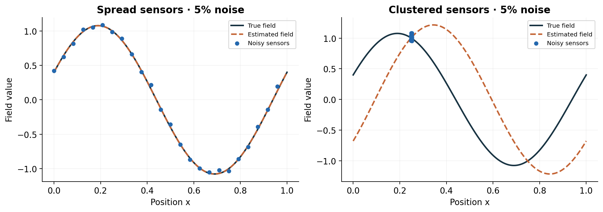
A fixed example from the new synthetic study (seed 7300). Distributed sensors constrain both modes; clustered observations provide poor information about the field away from the cluster. The dashed estimate still satisfies the supplied Helmholtz equation. Axis ranges are chosen independently so the failed estimate is visible.

At 5% noise, distributed-sensor errors range from 0.00116 to 0.02615, whereas clustered-sensor errors range from 0.1148 to 3.2584. Thus exact satisfaction of the equation coexists with large uncertainty in its solution. The noiseless omitted-mode check has relative field error 0.1825 despite a zero residual for the fitted two-mode equation. Increasing measurement precision cannot remove this representation bias.

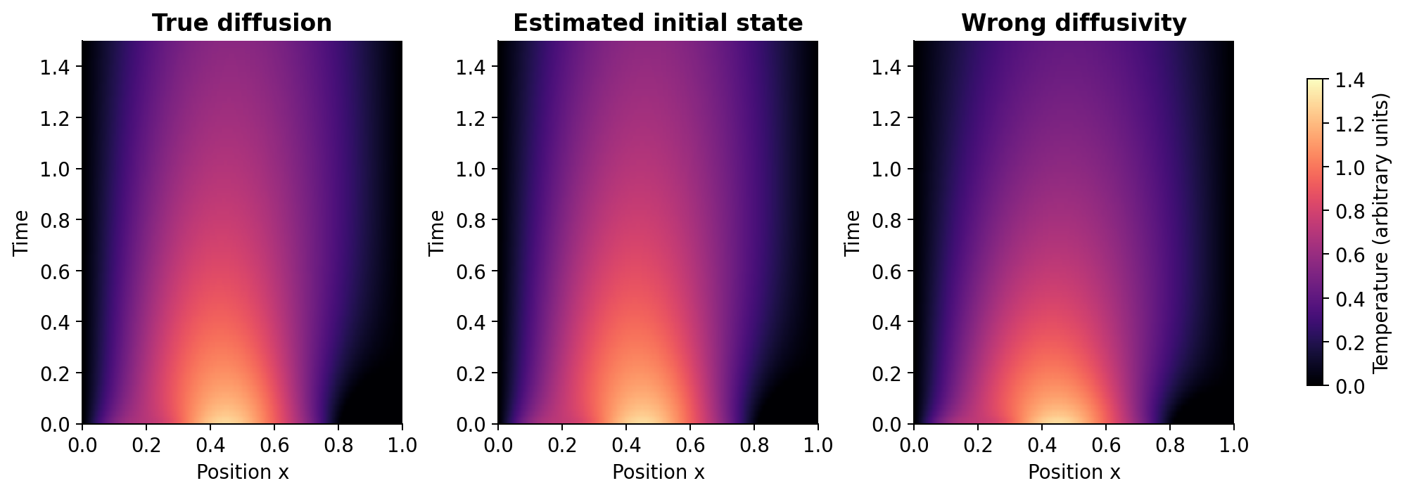
New six-mode heat study. The first panel is the true field, the second propagates an estimated initial state with the correct diffusivity, and the third uses the same estimated state with diffusivity 0.06 instead of 0.04. All panels use one temperature scale. The third case matches the second at time zero but diverges during prediction.

The heat example has relative space-time error 0.02091 with matched diffusivity and 0.12766 with the wrong diffusivity. The boundary values remain zero to floating-point precision in both models. Noise suppression through forward diffusion is therefore compatible with substantial model bias; boundary satisfaction alone is not a validation criterion.

Archived CPU panel, retained as a scoped implementation observation. Direct solution time and PINN training time are different workloads.
Method	Field RMSE	Recorded time
Full periodic FFT solve	1.9704 × 10⁻⁷	0.1695 ms per solve
Sine-network PINN, 1800 epochs	0.2120	109.112 s training

The full-grid FFT result is consistent with the supplied discrete operator being inverted directly. The much poorer PINN result motivates checking the computational formulation first, but does not distinguish architecture, optimization, boundary mismatch, and information access. The low-mode record remains in the supplement; it is not used as a headline. No comparison with a strong classical PDE solver would make the FFT path novel, since it is itself that classical solver.

9. Learning what the operator does not specify

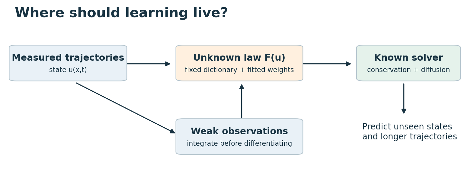
u_t=\nu u_{xx}-\partial_x F(u),\qquad F(u)=\sum_j\theta_j\psi_j(u).

A different placement of learning, implemented in the separate constitutive-law studies: observations constrain a small unknown flux inside a supplied conservation-and-diffusion solver. Weak observation equations integrate the data before estimating coefficients. This is not the architecture of the fixed Helmholtz experiment.

For a viscous conservation law, a fixed expansion of the unknown flux is linear in its coefficients even though the state evolution is nonlinear. This shifts learning from the complete state derivative to a physical component. The companion constitutive study [7] reports a median extrapolation error of 9.29 × 10⁻⁷ for a dictionary-matched oscillatory law, but 0.00520 for a saturating law outside the dictionary. A weak polynomial control also beats the richer weak dictionary at the higher reported noise setting. These results are separate archived experiments; they are not pooled with the new sensor study.

The architecture supplies a concrete research path: encode trustworthy conservation and boundary structure; identify the uncertain law using informative observations; propagate the assembled model; and evaluate prediction outside the fitting conditions. Local spline support and exact quadratic forms can help within that path, but a matched dictionary or a classical spectral solver can succeed without demonstrating a spline-specific contribution.

10. Discussion and reproducibility

The benefit of an operator-structured model is the removal of unnecessary degrees of freedom and repeated residual enforcement when the assumptions hold. Its liabilities are equally structural: a supplied basis may exclude the true field, poor sensor geometry may leave admissible solutions indistinguishable, and a misspecified operator may propagate an initially plausible state incorrectly. Deep networks remain relevant when representations, latent state, or nonlinear constitutive structure must be learned; the present calculations do not eliminate those problems.

All new calculations are deterministic, CPU-only, and bounded. The supplement records every noise-draw error, seeds, conditioning, analytic checks, and hashes of historical sources. The accompanying rebuild script generates the figures and browser data without neural training. The historical source is preserved separately and its timing metadata is incomplete. No measured neural trajectories have been reconstructed from aggregate metrics. The work supports a methodological distinction and reproducible small examples; it does not establish a practical deployment, SOTA superiority, or a new general PDE solver.

11. Conclusion

Known linear physics can be made an invariant of a model rather than a term repeatedly optimized. The remaining task is still statistical: observations must identify the admissible solution, and the encoded operator must describe the process. The sensor and heat experiments make these two requirements visible, while the constitutive architecture shows how the same separation extends toward genuinely unknown physics. The resulting design principle is to assign computation and learning to the uncertainties they actually resolve.

References

M. Raissi, P. Perdikaris, and G. E. Karniadakis. Physics Informed Deep Learning (Part I): Data-driven Solutions of Nonlinear Partial Differential Equations. 2017. Source
L. N. Trefethen. Spectral Methods in MATLAB. SIAM, 2000. Source
M. Unser and T. Blu. Cardinal Exponential Splines: Part I - Theory and Filtering Algorithms. IEEE Transactions on Signal Processing, 53(4), 1425-1438, 2005. Source
A. Badoual, D. Schmitter, and M. Unser. An Inner-Product Calculus for Periodic Functions and Curves. IEEE Signal Processing Letters, 23(6), 878-882, 2016. Source
S. L. Brunton, J. L. Proctor, and J. N. Kutz. Discovering governing equations from data by sparse identification of nonlinear dynamical systems. PNAS, 113(15), 3932-3937, 2016. Source
F. Black and M. Scholes. The Pricing of Options and Corporate Liabilities. Journal of Political Economy, 81(3), 637-654, 1973. Source
D. Schmitter. Learning Constitutive Laws Inside Known Dynamics: Structured Identification and Out-of-Range Prediction. Companion manuscript M03, 2026. Source