The goal is a useful onboard component
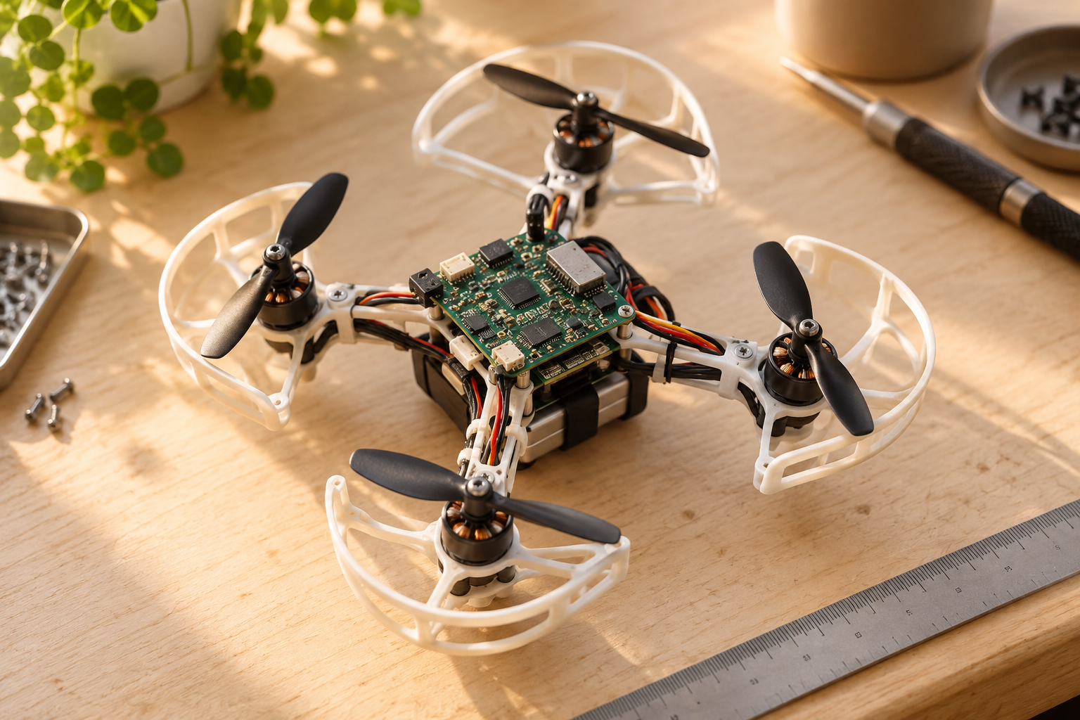
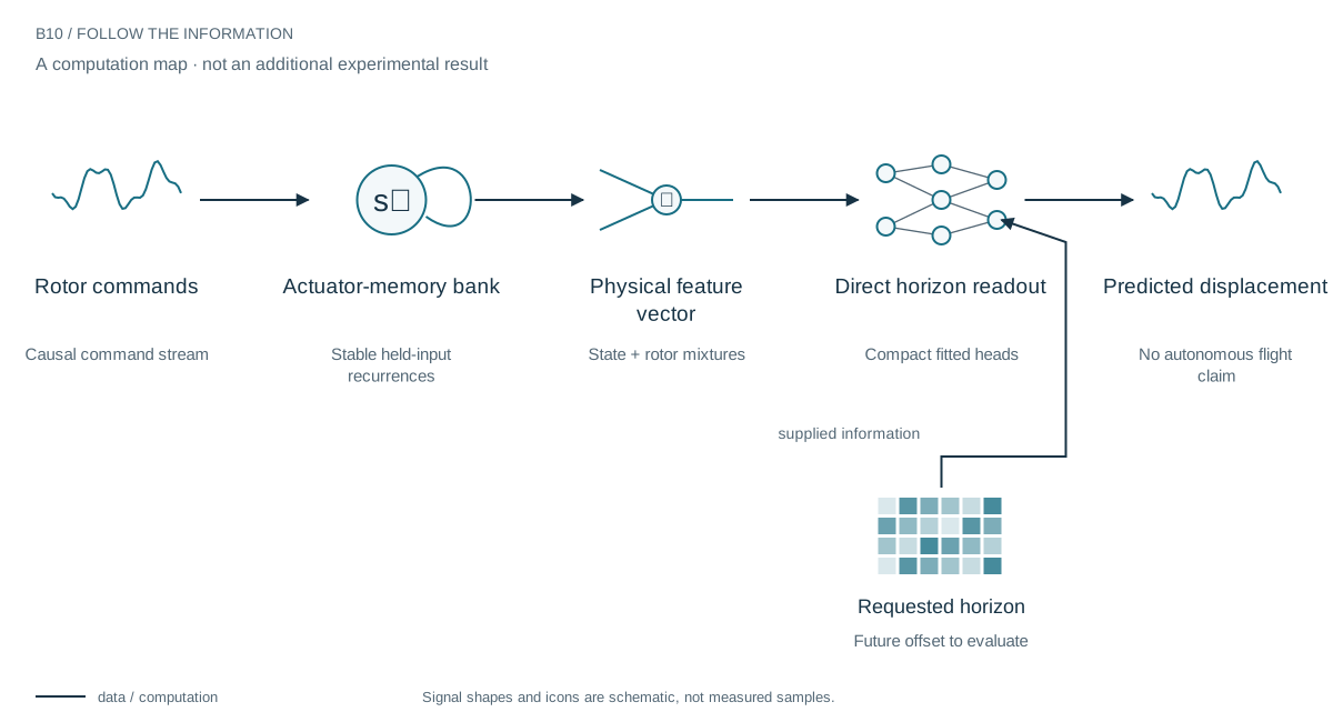
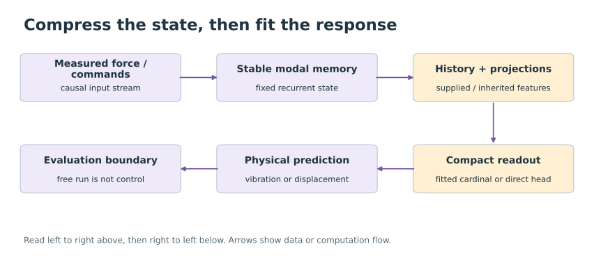
A small aircraft has little room for computation, but modeling its dynamics can require memory of past motor commands and several physical outputs. Our program uses exact sampled actuator-memory recurrences, rotor mixtures, and direct horizon-dependent readouts. It predicts displacement; it does not autonomously fly the drone.
Separate the tiny program from the entire learner
The compact drone model predicts displacement over a requested horizon from causal traces and physical features. It does not recursively feed its predicted future state back through fifty steps of the same learned network. That direct interface is part of its computational advantage and part of its limitation.
The strong comparison adapts a released neural ensemble on a related sparse endpoint task. The operator program is far smaller and cheaper to fit, but its four groups of physical errors are all worse. A later hybrid uses teacher execution statistics and different translation/angular components; its improved accuracy comes with additional inherited learning and prior exposure.
A strong comparator changed the headline
An early comparison looked favorable against published numbers under different observation protocols. The later study reproduced a released ASIA neural ensemble and adapted both approaches using corresponding sparse Melon-flight tasks. On the same 130 run-three starts, the adapted neural model wins position, velocity, orientation, and angular-velocity accuracy. That is the relevant accuracy conclusion.
The resource difference is still substantial
The compact program retains 24,288 bytes versus about 24.79 MB for the source-plus-adapted neural programs—roughly 1,020 times less. Measured compilation takes 1.538 seconds versus 101.33 seconds of target optimization. Label counts are close but unequal: 3,250 versus 3,380. These are program and fitting measurements, not total runtime RSS, battery consumption, or weak-device timing.
Combining mechanisms helped, with a remaining gap
A later post-exposure program uses a recurrent model for translation and direct heads for angular outputs. It consolidates pseudo-experience from more than one teacher execution through additive Grams. Its mean physical error ratio to the adapted ensemble becomes 1.1218, while retained size remains about 314 times smaller. The teacher disappears at runtime but its acquisition cost is not free.
Find the application on the error–resource frontier
For an onboard use case, the question is whether this error–resource tradeoff meets a real tolerance: perhaps a monitoring estimate, a planning approximation, or a fallback model. The archive has not tested that decision. The scientific result is a measured frontier and an explanation of what the small program contains—not a demonstration that a tiny network can replace the drone controller.
The meaningful frontier
A deployment may accept a small accuracy cost to obtain a much smaller model; another may not. Neither answer can be chosen from a compression ratio alone. The next application would need to show that the compact model meets the controller’s actual tolerance on the intended hardware. The current paper establishes a predictive accuracy–resource tradeoff, not a flight-control breakthrough.
Evidence & further reading
The links below distinguish the project record from foundational literature. This revised story does not add a new application-validation experiment.
- Consolidated research results, including constitutive edges and continual memory. Daniel Schmitter (2026). Local archive snapshot.
- Consolidated limitations and research boundaries. Daniel Schmitter (2026). Local archive snapshot.
- Experiment-family evidence map. Spline research archive (2026). Local archive snapshot.