Precision has a shape
Suppose two option positions largely offset each other. Bounding each position’s numerical error separately and then adding the bounds is safe, but it may discard exactly the structure that makes the portfolio small. The same issue appears when subtracting nearby predictions, computing a sensitivity, or comparing two continuous models. The output is a signed functional, not a bag of unrelated values.
Ask for the portfolio response directly
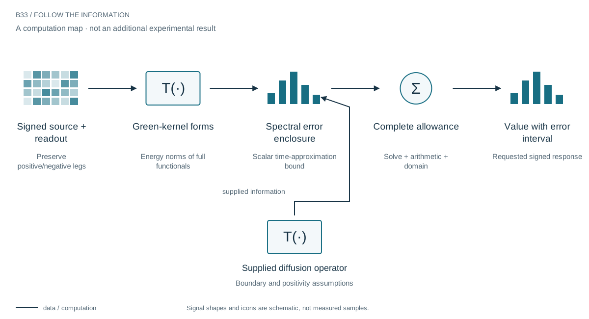
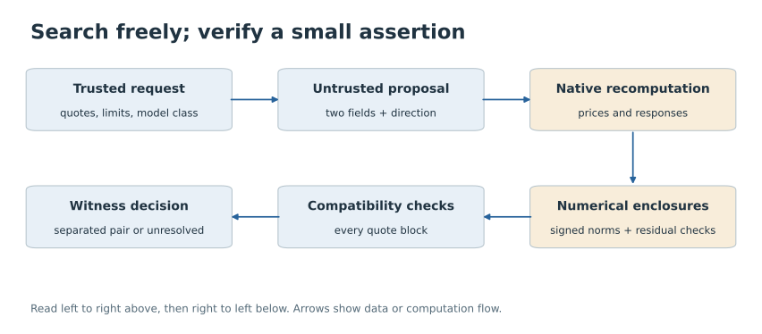
A spread is a signed combination of payoffs. A finite spot response is another signed combination of readouts. Bounding each atom first throws away cancellation. The operator energy norm instead evaluates a small Green-kernel quadratic form on each complete signed functional, then combines those norms with a scalar time-inversion error bound.
The resulting allowance follows the requested output rather than the largest individual component. Its tightness gain is not the same as a latency gain. Boundary assumptions and outward arithmetic still have to be included before the value becomes a usable numerical enclosure.
Use the geometry of the operator
For the declared diffusion, a spectral argument transfers a scalar time-approximation error to an output error through two energy norms: one for the source and one for the readout. Each norm is a signed quadratic form in a Green kernel. Opposite-sign terms are combined inside that form, before any triangle inequality throws their cancellation away.
A bound over the spectrum, not a sampled check
The implementation encloses the scalar approximation error over the entire nonnegative spectrum using interval Taylor expansions and a tail treatment. It then adds validated solve, arithmetic, and any applicable domain allowances. Agreement on a handful of eigenvalues would be a diagnostic, not the same guarantee. Exact spatial cells remove one approximation source but do not make floating-point computation exact.
What improved
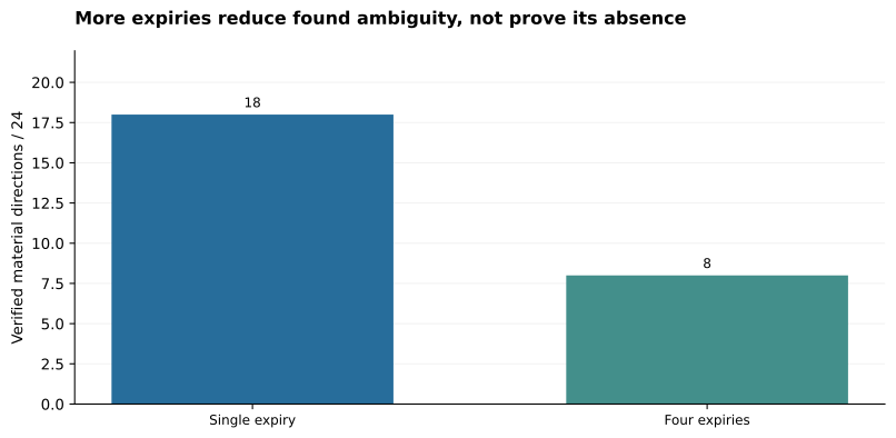
In the initial signed-output example, this transfer is about 172 times tighter than separately accumulating leg bounds. That is a tighter guarantee, not a 172-times runtime speedup. A later fresh panel contains the independent reference in all 320 field/maturity cases. Its assumptions still include a bounded positive coefficient field, declared boundaries, and the specified arithmetic behavior.
An error budget shaped like the requested output
For scientific ML and numerical services, the broader idea is output-aware assurance. A precise bound on the quantity a user asks for can be far more useful than a crude uniform bound on every intermediate field. This work implements that principle for a supplied one-dimensional pricing operator, not for arbitrary neural outputs.
A useful interface for numerical intelligence
A learned system can propose a physical model or request a response; a numerical component can return both the value and the uncertainty caused by its computation. This does not quantify every modeling error, and it does not certify that the world obeys the supplied equation. Its value is narrower and tangible: subsequent decisions need not confuse a precise-looking decimal with a numerically justified one.
Evidence & further reading
The links below distinguish the project record from foundational literature. This revised story does not add a new application-validation experiment.
- Compact, verifiable operator-based options risk. Spline research archive (2026). Local archive snapshot.
- Compact operator representations for option pricing and risk. Spline research archive (2026). Local archive snapshot.
- Single-thread deployment succeeds on the shared workstation. Spline research archive (2026). Local archive snapshot.