The instability is in the coordinates
Consider the difference between two exponential responses divided by the distance between their poles. As the poles meet, the expression has a perfectly finite derivative limit. Computing two nearly equal exponentials and subtracting them can nevertheless lose precision. Worse, an expanded representation may store very large opposite-sign coefficients even though their sum is modest.
A pole collision changes the best coordinates
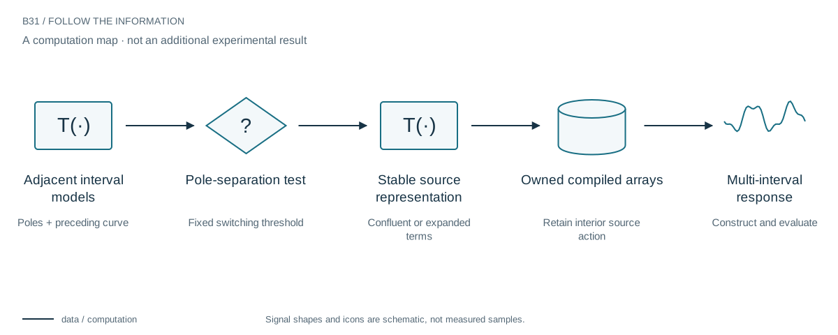
When one maturity interval is forced by the preceding curve, the source contains more information than two endpoints. Distinct-pole expansions can encode a smooth limit using huge coefficients of opposite signs. Near a collision, evaluating those terms separately loses digits before they cancel.
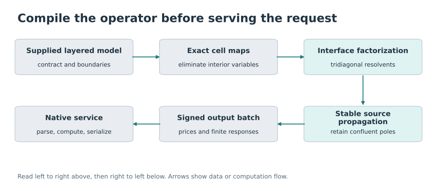
The compiled representation instead retains the divided difference as one object and uses a parameter derivative in the repeated-pole limit. Only well-separated pairs are expanded. This is a change in numerical representation, not a lossy fit of the preceding solution or a new physical model.
Keep the collision as a first-class object
Repeated roots naturally produce polynomial-times-exponential functions. Hermite and confluent representations keep that structure intact instead of pretending that two almost-equal roots are comfortably distinct. In the pricing implementation, close operator pairs retain a stable divided difference; sufficiently separated pairs use ordinary expanded terms. The switching threshold was fixed before the comparison.
Why this becomes important across time
With several volatility intervals, the solution from one interval becomes a source for the next. Endpoint values alone do not describe that source. Exact cross-operator products preserve its interior contribution, but a naive chain repeatedly re-evaluates earlier objects. The compiled representation owns the necessary source arrays and avoids that recursive overhead. Stability and execution cost are linked through the same choice of coordinates.
What the complete test says
All twelve prescribed three-interval cases pass the accuracy checks. Complete construction and evaluation fall from 63–117 milliseconds to 4–12 milliseconds, a paired internal gain of 5.30–17.18 times. These are comparisons of two implementations of the same calculation, not a victory over the financial-software field. The separate artifact budget fails: 132,999 bytes exceed the declared 102,400-byte limit.

Make limiting configurations first-class objects
The complete multi-interval study shows a substantial internal speed gain from selective confluence and owned source arrays, while failing its artifact-storage budget. Both belong in the result. The transferable idea is to treat limiting configurations as first-class numerical objects rather than hoping ordinary coefficients remain well conditioned.
A transferable numerical habit
The gain is not that exponentials are always better than polynomials. It is that the representation should stay well-conditioned as the physical parameters move. Learned poles, nearly repeated modes, and changing dynamical models can all encounter this issue. A mathematically harmless limit deserves a numerically harmless implementation—and a benchmark that includes preparation, not only the final evaluation.
Evidence & further reading
The links below distinguish the project record from foundational literature. This revised story does not add a new application-validation experiment.
- Compact operator representations for option pricing and risk. Spline research archive (2026). Local archive snapshot.
- Compact, verifiable operator-based options risk. Spline research archive (2026). Local archive snapshot.
- Operator-spline theory: consolidated research manuscript. Daniel Schmitter (2026). Local archive snapshot.