What if the model already knows the local answer?
A conventional numerical grid spends unknowns throughout a domain. A physics-informed neural network instead spends parameters and optimization steps representing a solution. Both are general approaches. But when the equation inside each region has a known analytic solution, another option appears: represent exactly what can happen inside that region and solve only for how neighboring regions connect.
The network analogy is a compiler, not a neural surrogate
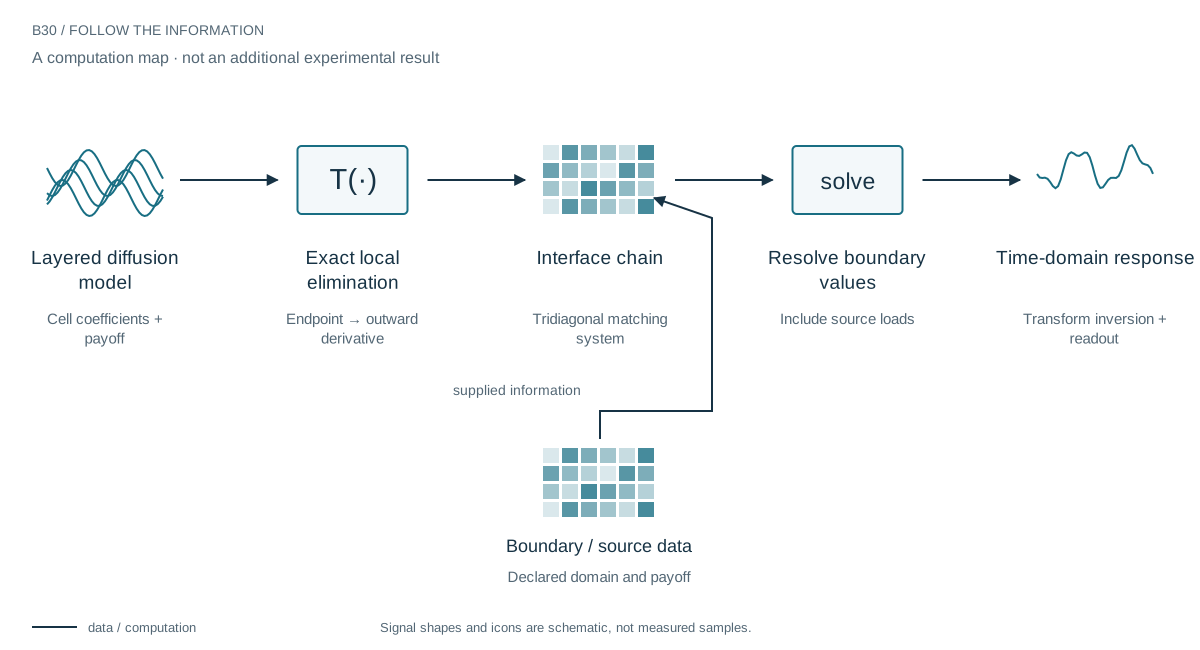
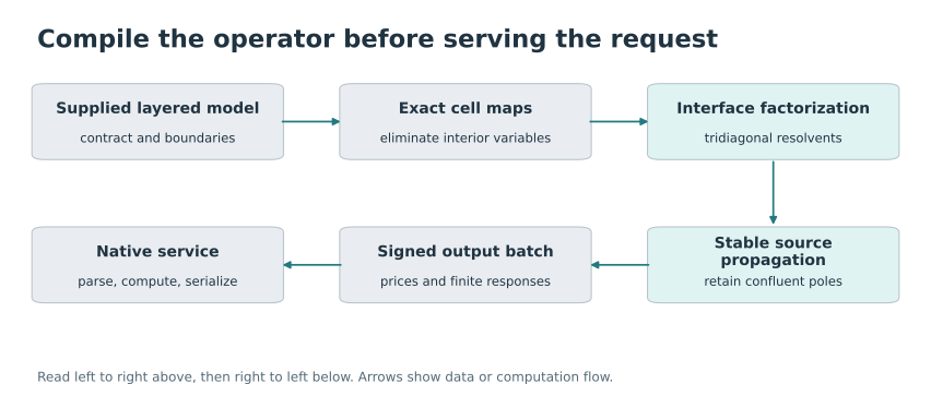
Inside one constant-coefficient cell, the differential operator supplies the complete homogeneous shape. Endpoint values are its coordinates. Matching outward derivatives connects neighboring cells into a small interface system, and payoff sources add known loads. The cell interior does not need a fine spatial grid of learned or numerical unknowns.
This resembles an ML layer whose fixed features encode supplied physics and whose coefficients are solved from constraints. In this application there is no trained neural pricing model. The benefits come from exact local elimination and reuse across a batch of readouts, with time-inversion and arithmetic errors handled separately.
Two numbers can describe a whole cell
After a time transform, our layered European pricing problem has constant coefficients within each spatial cell. Two endpoint values determine its homogeneous interior. A two-by-two matrix maps those values to outward derivatives. Matching the derivatives across interfaces produces a tridiagonal chain. Local source terms need their own correction; discarding them would make the representation incomplete.
The link to operator-based learning
The principle is the same one that makes operator-matched spline spaces attractive: choose coordinates adapted to the equation before asking an optimizer or solver to work. Here the financial cells are heterogeneous and nonuniform, not a cardinal spline grid. Their benefit comes from exact local elimination and reusable boundary algebra—not from attaching the spline name to a standard matrix solve.
The workload determines the winner
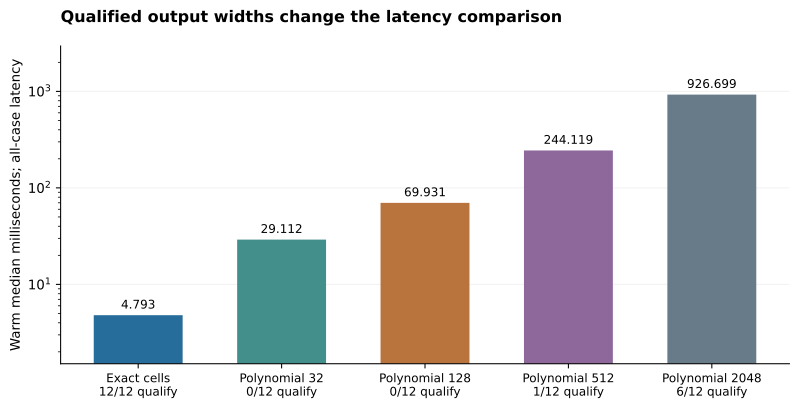
A model service may answer hundreds of strikes after every coefficient update, or just query an already-prepared curve. Those are different jobs. In the archive, a prepared polynomial interpolant is faster for 501 isolated queries. Exact cells are competitive when reconstruction is included. Selected inverse rows help batches but usually lose the one-contract comparison. The paper keeps these boundaries visible.
A small operator engine for changing models
The service vision is repeated conditional pricing after a model changes, on modest runtime resources. It is not discovering the correct market model. The workload decides whether exact cells help: a prepared ordinary curve can be faster for warm queries, while reconstruction-plus-query work is a different comparison.
A small engine is not the whole application
The native implementation returns enclosed outputs using modest runtime memory, but only for its declared supplied diffusion model. It does not handle every exotic contract, infer a valid market model, or demonstrate a trading advantage. The interesting general lesson is computational: a good local solution space can remove work before acceleration begins. That idea applies to learned physical components whenever their mathematical structure genuinely permits it.
Evidence & further reading
The links below distinguish the project record from foundational literature. This revised story does not add a new application-validation experiment.
- Compact operator representations for option pricing and risk. Spline research archive (2026). Local archive snapshot.
- Compact, verifiable operator-based options risk. Spline research archive (2026). Local archive snapshot.
- Cardinal Exponential Splines: Part I—Theory and Filtering Algorithms. Michael Unser and Thierry Blu (2005). Primary literature.