The architecture in context
The system we are building
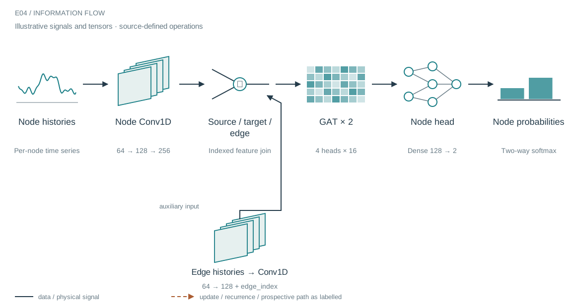
The graph model treats relationships as data, not just wiring. Node histories and edge histories pass through separate convolutional encoders. For each listed edge, the attention scorer combines source-node, destination-node and edge features. Multi-head aggregation then lets the model use several relational views before a node-level classifier.
Who does what in the stack
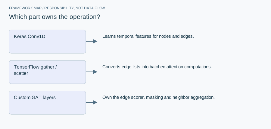
- Keras Conv1D
- Learns temporal features for nodes and edges.
- TensorFlow gather / scatter
- Converts edge lists into batched attention computations.
- Custom GAT layers
- Own the edge scorer, masking and neighbor aggregation.
Instead of calling a packaged graph library, the notebook implements gather, score, scatter and aggregation in TensorFlow. This makes the mechanism visible and accommodates custom edge features, but it also makes the author responsible for topology semantics, duplicate edges and isolated nodes.
Open up the implementation
Open up one graph-attention head
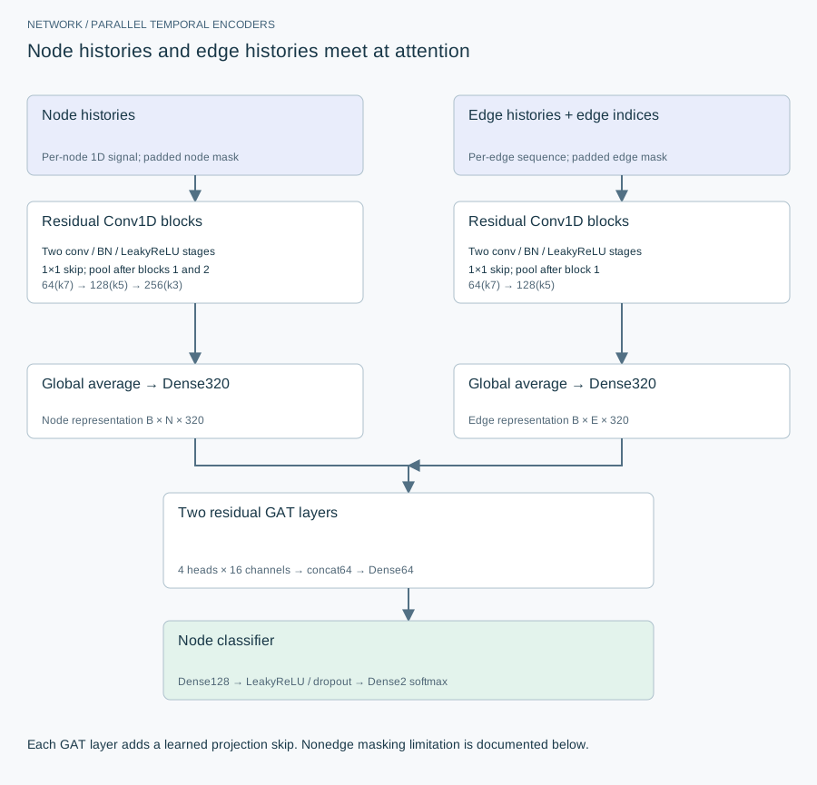
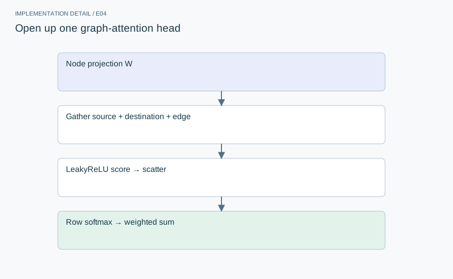
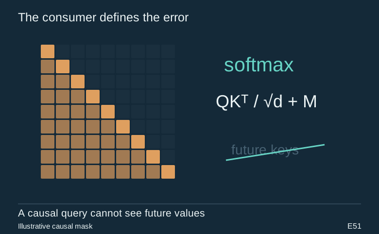
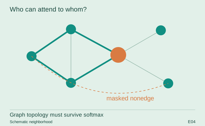
The node and edge encoders feed separate tensors to each GAT head. Each head projects node features, gathers both endpoints, concatenates edge features and computes a scalar compatibility. Head outputs concatenate before an output projection and LayerNorm. Unlike dot-product transformer attention, this score is an affine map of concatenated endpoint/edge features. The inspected implementation scatters scores into a dense N×N array: absent edges become zero logits. Softmax assigns them positive probability because the intended nonedge masking line is commented out.
The mathematical contract
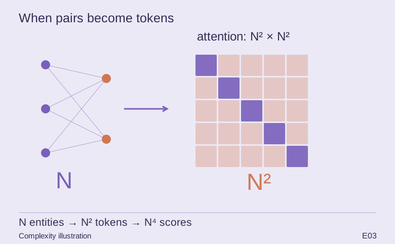
The correct engineering question is not simply how many heads fit in memory. It is whether the neighborhood represented by the adjacency data is the neighborhood actually used by normalization. Four heads split 64 channels here; increasing heads at fixed total width changes per-head expressivity. The dense scatter also retains quadratic storage even when the original edge list is sparse.
Implementation and resource card
- Capacity / budget
- Training cell:4 heads, total hidden width 64 (16 per head),2 output classes, dropout .2, batch 64, maximum 200 epochs, Adam learning rate 1e-5. No verified total count or convergence time is attached.
- Execution evidence
- This revision inspects and explains the archived implementation. It does not rerun the original workload. No unrecorded convergence time, throughput or accelerator result is supplied.
- Current reproduction context
- Current workstation, supplied by the author: Apple M4, 128 GB unified RAM, 40 GPU cores and 16 CPU cores. This is context for prospective reproduction, not attribution of every archived run. Python and framework versions are not fully locked for these historical sources; declarations, when available, are identified separately.
From explanation to a reproducible check
Build a graph with three nodes and only one directed edge. Inspect the complete attention matrix before and after softmax. Mark the existing behavior and any repaired masked version separately. For a masked repair, define isolated-node behavior and self-loops explicitly; an all-masked row needs a policy, not an accidental NaN.
Preserve input identities, configuration and failure records with the result. A successful numerical check only establishes the operation it exercises: it does not certify an entire dataset, model or deployed system. Reproduce the interface on a small deterministic input before optimizing throughput or increasing workload size.
A closer look at the implementation
The code that carries the idea
The snippet scatters edge logits into a dense B × N × N matrix and applies softmax. Unlisted entries are initialized to zero by scatter_nd. Zero is a perfectly valid logit: after softmax it receives positive probability. The commented-out masking line is not active code, and masking every numerical zero would also erase legitimate zero-scored edges.
        attention_matrix = tf.scatter_nd(
            scattered_indices,
            attention_scores,
            [batch_size, num_nodes, num_nodes]
        )

        # Add numerical stability to softmax
        attention_matrix = tf.clip_by_value(attention_matrix, -1e9, 1e9)

        # Add small epsilon and mask invalid entries
        #attention_matrix = attention_matrix + (tf.cast(tf.equal(attention_matrix, 0), tf.float32) * -1e9)

        # Apply softmax
        attention_weights = tf.nn.softmax(attention_matrix, axis=-1)
Verbatim archive excerpt from gat_model.ipynb. Context-dependent historical code, not a standalone runnable program. Comments retain their original wording; the article distinguishes implemented behavior from stale or overbroad comments.
The boundary that matters
As written, this layer does not guarantee attention only over listed neighbors. A repair would construct a separate boolean adjacency mask and define an isolated-node policy. That repair is a proposed engineering change, not silently substituted into the archived excerpt or claimed as a validated experiment.