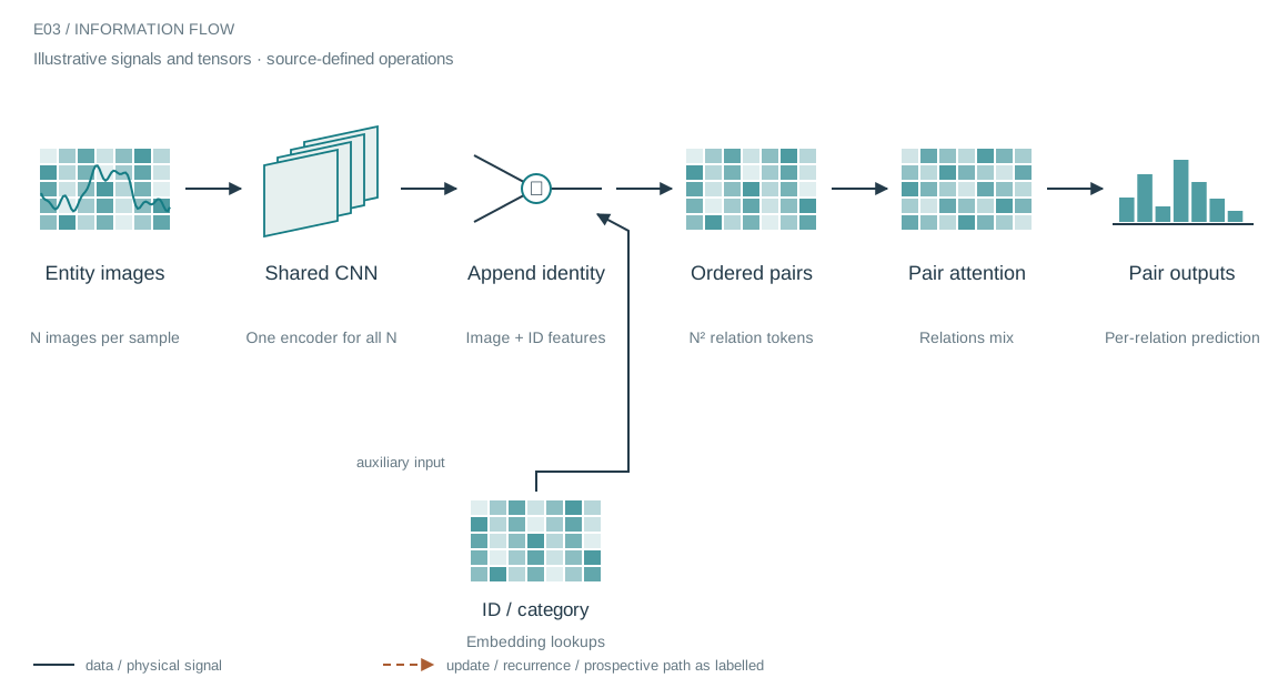
The architecture in context
The system we are building
An entity’s local image can be encoded once and reused across its relationships. This notebook applies the same CNN to each entity, combines visual features with identity and category embeddings, then constructs ordered pairs. The pair representation can distinguish “A relative to B” from “B relative to A”; that directionality would disappear under a symmetric sum.
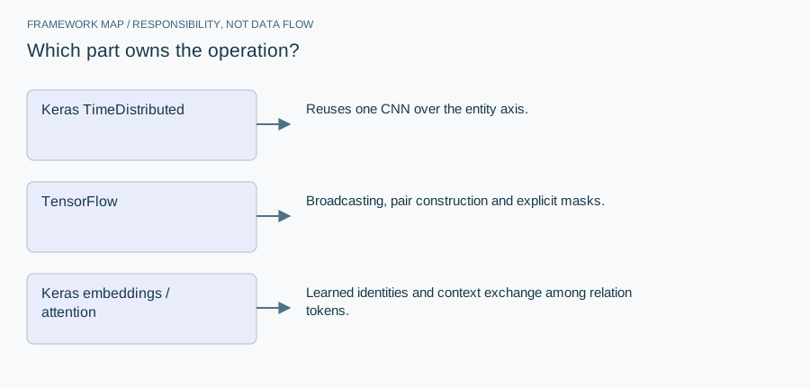
Who does what in the stack
- Keras TimeDistributed
- Reuses one CNN over the entity axis.
- TensorFlow
- Broadcasting, pair construction and explicit masks.
- Keras embeddings / attention
- Learned identities and context exchange among relation tokens.
Custom MaskLayer, PairwiseFeatureLayer and PairwiseMaskLayer bridge a set-shaped input and Keras attention. The custom work is data layout and relation construction, not a new attention primitive. The generator supplies padded daily groups, so missing entities and genuine low-valued measurements must remain distinguishable.
From module map to executable structure
Inside Shared CNN with pairwise attention
N padded instruments, 25 × 31 grayscale images; embedding width 32; one attention head with key_dim 32.
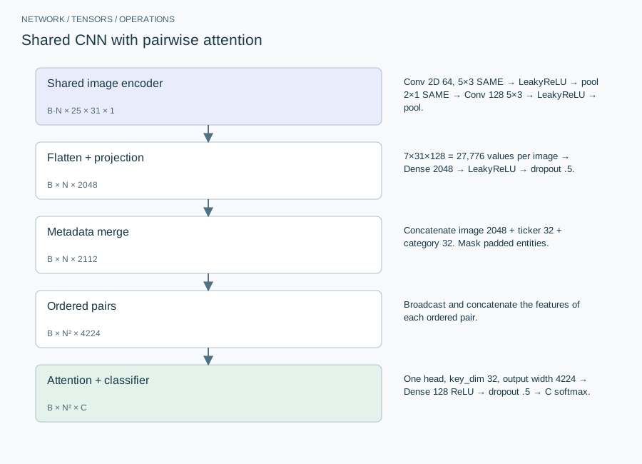
| Layer or branch | Output shape | Implementation detail |
|---|---|---|
| Shared image encoder | B·N × 25 × 31 × 1 | Conv 2D 64, 5×3 SAME → LeakyReLU → pool 2×1 SAME → Conv 128 5×3 → LeakyReLU → pool. |
| Flatten + projection | B × N × 2048 | 7×31×128 = 27,776 values per image → Dense 2048 → LeakyReLU → dropout .5. |
| Metadata merge | B × N × 2112 | Concatenate image 2048 + ticker 32 + category 32. Mask padded entities. |
| Ordered pairs | B × N² × 4224 | Broadcast and concatenate the features of each ordered pair. |
| Attention + classifier | B × N² × C | One head, key_dim 32, output width 4224 → Dense 128 ReLU → dropout .5 → C softmax. |
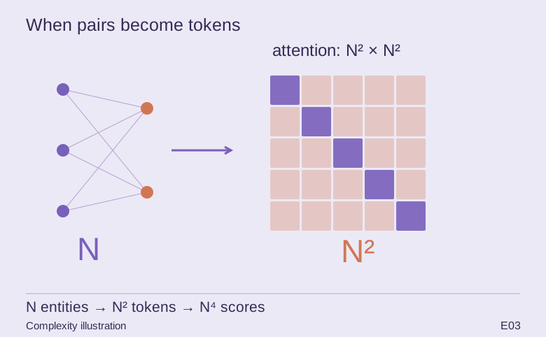
Pairs are tokens, rather than pairs being individual attention edges. With N entities there are N² tokens, and dense attention over them can require N⁴ scores per head. Sharing the CNN avoids N separate parameter sets but does not remove this pairwise activation cost. The flattened image projection, not the single attention head, dominates the encoder’s stored weights.
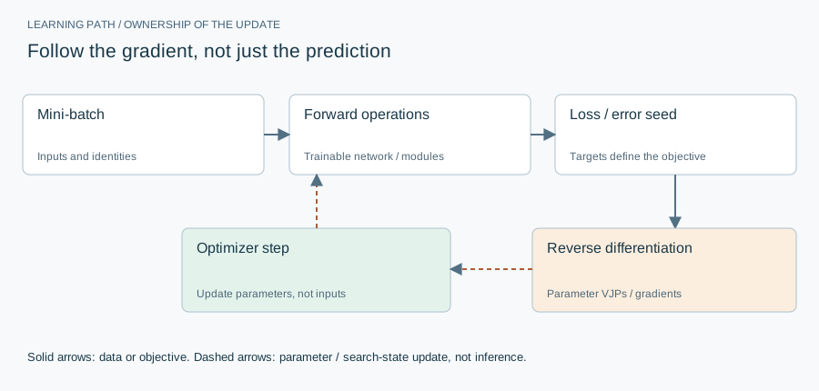
The equation and the update
The notebook selects batch size 1 and Adam with gradient-norm clipping. Per-pair classification requires the padding mask to enter both attention and the loss denominator; zero feature vectors alone do not establish that contract.
Implementation card / no invented benchmarks
Capacity, budget and execution evidence
- Parameters / retained state
- The image encoder alone has 57,011,328 parameters, including biases. Total also depends on ticker vocabulary and class count; not inferred as a fixed number.
- Duration and hardware evidence
- No verified full-run duration in this card; batch size 1 is a configuration, not an efficiency result.
- Source coordinates
- E03 cell 8, lines 163–248; configuration at its start
- Current reproduction context
- Current workstation, supplied by the author: Apple M4, 128 GB unified RAM, 40 GPU cores and 16 CPU cores. This is context for prospective reproduction, not attribution of every archived run. Python and framework versions are not fully locked for these historical sources; declarations, when available, are identified separately.
Counts above are calculated from the stated layer shapes unless identified as saved measurements. They exclude optimizer state and nontrainable buffers. No archived training was rerun for this revision.
What these design choices change
The 2048-wide image projection retains far more capacity than a pooled 128-channel alternative. Replacing it with global pooling is a redesign, not a free acceleration: it changes which spatial patterns can survive. Similarly, selecting sparse pairs changes the task’s coverage. Benchmark such alternatives with the same entity set and explicitly report excluded pairs.
Reproduction and measurement protocol
Construct a two-entity batch plus padding. Trace the ordered pairs (0,0), (0,1), (1,0), (1,1), their targets and their validity masks. Inspect the attention mask’s query and key axes rather than assuming a squeezed token mask broadcasts as intended. Changing a padded entity must not change valid predictions when masking is correct.
For a new run, save the resolved Python/framework versions, backend, dtype, seed, input shapes, batch size and exact source revision. Start with one batch and one update. Log training steps separately from epochs or environment steps. Do not equate the configured maximum with a completed budget or convergence.
Measure initialization/compilation, data preparation, warmed forward pass, training updates and evaluation separately. Synchronize accelerator work around timed regions using the chosen framework’s supported mechanism. Report peak process memory and framework allocation separately; parameter bytes exclude activations, gradients, optimizer state and input buffers. On a shared machine, begin with a single CPU worker and a small batch rather than claiming all available resources.
A closer look at the implementation
The code that carries the idea
The excerpt expands the feature tensor along two different axes, tiles both views and concatenates them. Its output has N² tokens, each containing two D-dimensional entity vectors. This is easy to inspect but materializes the pair tensor. If full attention is then applied over all those tokens, its score matrix can grow as N⁴—not merely N².
class PairwiseFeatureLayer(tf.keras.layers.Layer):
    def call(self, inputs):
        batch_size = tf.shape(inputs)[0]
        n_tickers = tf.shape(inputs)[1]
        feature_dim = tf.shape(inputs)[2]

        # Create pairwise combinations using broadcasting
        # Expand dims for broadcasting: (batch, n_tickers, 1, features) and (batch, 1, n_tickers, features)
        features_i = tf.expand_dims(inputs, axis=2)  # Shape: (batch, n_tickers, 1, features)
        features_j = tf.expand_dims(inputs, axis=1)  # Shape: (batch, 1, n_tickers, features)

        # Tile to create all pairs
        features_i = tf.tile(features_i, [1, 1, n_tickers, 1])  # Shape: (batch, n_tickers, n_tickers, features)
        features_j = tf.tile(features_j, [1, n_tickers, 1, 1])  # Shape: (batch, n_tickers, n_tickers, features)

        # Concatenate along feature dimension
        pairwise_features = tf.concat([features_i, features_j], axis=-1)  # Shape: (batch, n_tickers, n_tickers, 2*features)

        # Reshape to expected output shape
        pairwise_features = tf.reshape(pairwise_features,
                                     [batch_size, n_tickers * n_tickers, 2 * feature_dim])

        return pairwise_features
Verbatim archive excerpt from cnn_self_attention_model_b_opt_lp2.ipynb. Context-dependent historical code, not a standalone runnable program. Comments retain their original wording; the article distinguishes implemented behavior from stale or overbroad comments.
The boundary that matters
Multiplying an embedding by zero does not by itself forbid attention to that entity. The archived pair mask must be checked against the attention layer’s query–key mask shape. Do not assume a flattened validity vector expresses every prohibited pairwise interaction.