The architecture in context
The system we are building
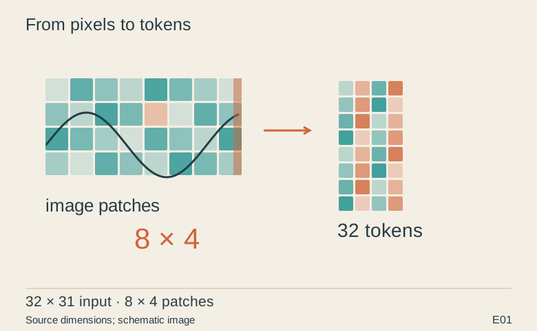
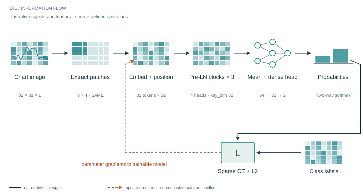
A small image need not go through a large vision backbone. This notebook divides a chart into rectangular patches, projects each patch into a learned token space, adds position embeddings and lets self-attention exchange context. The long and short patch dimensions encode a deliberate view of the image: a patch is a local unit of evidence, not an arbitrary flattening of the whole chart. With SAME padding, the 31-pixel width contributes eight patch columns rather than losing its right edge.
Who does what in the stack
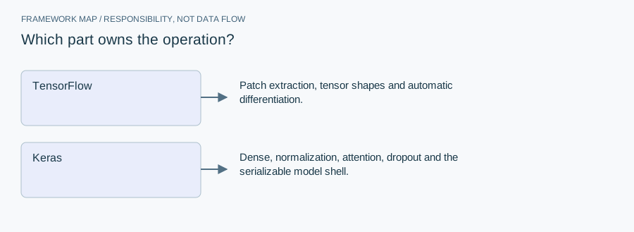
- TensorFlow
- Patch extraction, tensor shapes and automatic differentiation.
- Keras
- Dense, normalization, attention, dropout and the serializable model shell.
The custom Keras model assembles patch extraction, position embeddings and three explicit pre-normalized residual blocks. It then averages the tokens before classification. TensorFlow supplies tensor operations and differentiation; Keras supplies trainable layers and model configuration. This is application-level composition, not a modification of TensorFlow itself.
From module map to executable structure
Inside Keras patch transformer
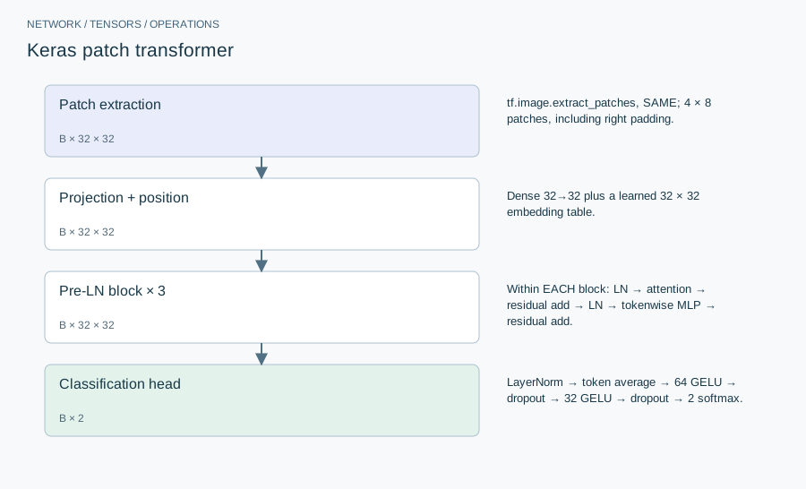
Training-cell configuration: 32 × 31 × 1 images, 8 × 4 patches, d=32, 4 heads, key_dim=32, 3 blocks.
| Layer or branch | Output shape | Implementation detail |
|---|---|---|
| Patch extraction | B × 32 × 32 | tf.image.extract_patches, SAME; 4 × 8 patches, including right padding. |
| Projection + position | B × 32 × 32 | Dense 32→32 plus a learned 32 × 32 embedding table. |
| Pre-LN attention × 3 | B × 32 × 32 | LayerNorm → Q/K/V → 4 heads of width 32 → concat 128 → output projection 32 → residual add. |
| MLP inside each block | B × 32 × 32 | LayerNorm → Dense 64 → GELU → dropout .3 → Dense 32 → dropout .3 → residual add. |
| Classification head | B × 2 | LayerNorm → token average → 64 GELU → dropout → 32 GELU → dropout → 2 softmax. |
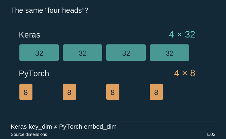
Both residual additions require the branch to return width 32. The attention branch temporarily expands to 128 channels because Keras key_dim is the width of each head, not the total embedding width. Its 4 score matrices are 32 × 32 per image. The MLP acts on each token separately; attention, not the MLP, mixes token positions. Averaging removes the token axis only after all three blocks.
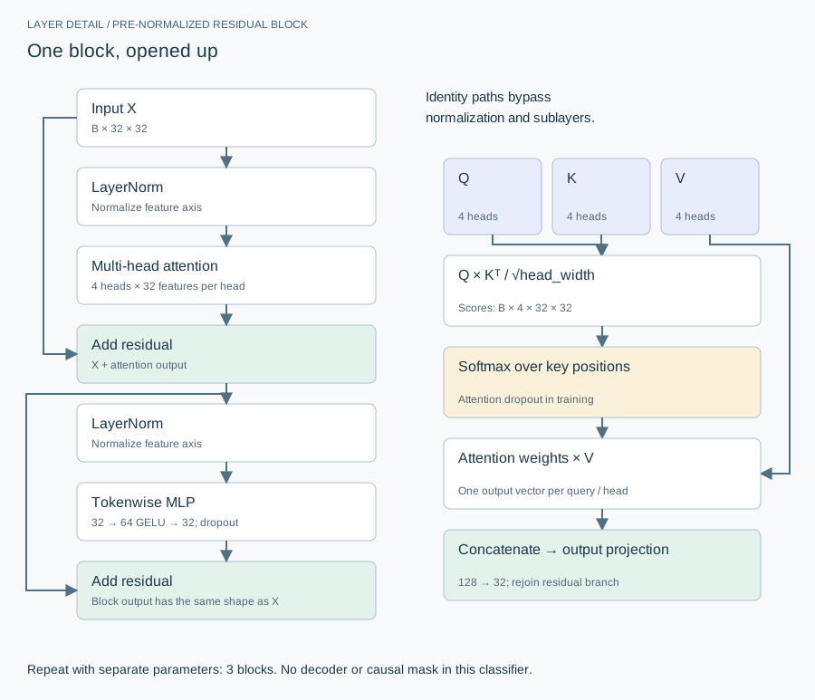
Diagram hierarchy informed by Figures 1–2 of Attention Is All You Need. Original figures here follow the archived classifier code; in particular its pre-LN placement differs from that paper’s post-LN architecture.
The equation and the update
Sparse categorical cross-entropy plus the two head kernels’ L2 penalties (1e-4). AdamW: learning rate 1e-5, weight decay 1e-5, elementwise gradient clipvalue 1.0; batch 256; maximum 200 epochs. Validation-loss early stopping: patience 40; plateau factor .8, patience 15, minimum rate 1e-7. Configured limits are not a convergence claim.
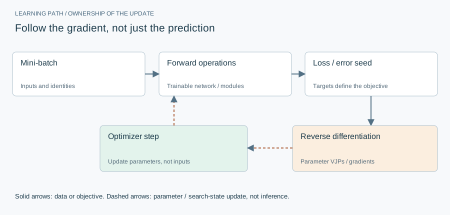
Implementation card / no invented benchmarks
Capacity, budget and execution evidence
- Parameters / retained state
- 69,762 trainable scalars; biases, position embeddings and normalization scale/offset included.
- Duration and hardware evidence
- No verified end-to-end training duration or workstation identity attached here. The training cell requests TensorFlow /GPU:0; this is not evidence of PyTorch MPS execution.
- Source coordinates
- E01 cell 2, lines 446–635; cells 4 and 6
- Current reproduction context
- Current workstation, supplied by the author: Apple M4, 128 GB unified RAM, 40 GPU cores and 16 CPU cores. This is context for prospective reproduction, not attribution of every archived run. Python and framework versions are not fully locked for these historical sources; declarations, when available, are identified separately.
Counts above are calculated from the stated layer shapes unless identified as saved measurements. They exclude optimizer state and nontrainable buffers. No archived training was rerun for this revision.
What these design choices change
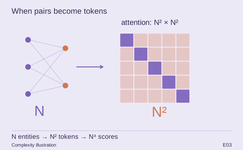
These are archived design choices, not an ablation-proven optimum. An 8 × 4 patch trades spatial detail for a short token sequence; halving both patch dimensions approximately quadruples token count and multiplies dense attention scores by sixteen. Global average pooling keeps the head independent of token count, but discards explicit position-specific features after contextualization. Wider heads change projection cost even when residual width stays fixed.
Reproduction and measurement protocol
Reimplementation order matters: verify padded patch order on a numbered image, test the positional table length, then check each residual shape before training. Feed integer labels to sparse cross-entropy; do not apply a second softmax to the probabilities. Keep the chronological date split and preprocessing fixed when comparing widths. The notebook’s informal ASCII architecture says 4 × 4 and Add & Normalize; the executable implementation uses 8 × 4 and pre-normalization. This article follows executable code.
For a new run, save the resolved Python/framework versions, backend, dtype, seed, input shapes, batch size and exact source revision. Start with one batch and one update. Log training steps separately from epochs or environment steps. Do not equate the configured maximum with a completed budget or convergence.
Measure initialization/compilation, data preparation, warmed forward pass, training updates and evaluation separately. Synchronize accelerator work around timed regions using the chosen framework’s supported mechanism. Report peak process memory and framework allocation separately; parameter bytes exclude activations, gradients, optimizer state and input buffers. On a shared machine, begin with a single CPU worker and a small batch rather than claiming all available resources.
A closer look at the implementation
The code that carries the idea
The excerpt is one complete residual block. Layer normalization precedes attention, the first addition preserves the incoming token stream, and the two dense layers create a separate feed-forward residual branch. The additions require matching final dimensions; the hidden expansion can be larger. The archived attention uses key_dim=32 with four heads: 32 is the size of each head, not the total four-head projection.
        y1 = self.norm1_1(x)
        y1 = self.attention1(y1, y1)
        x = x + y1

        y1 = self.norm1_2(x)
        y1 = self.dense1_1(y1)
        y1 = self.drop1_1(y1)
        y1 = self.dense1_2(y1)
        y1 = self.drop1_2(y1)
        x = x + y1
Verbatim archive excerpt from cnn_transformer_model_lp3_3class.ipynb. Context-dependent historical code, not a standalone runnable program. Comments retain their original wording; the article distinguishes implemented behavior from stale or overbroad comments.
The boundary that matters
The filename says “3class”, but the inspected model ends in two probabilities. Its saved training history is evidence of a historical run, not a new generalization test. The custom patch-count arithmetic also deserves a divisible-width test before reuse.