The architecture in context
The system we are building
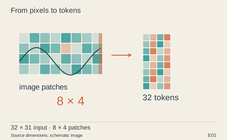
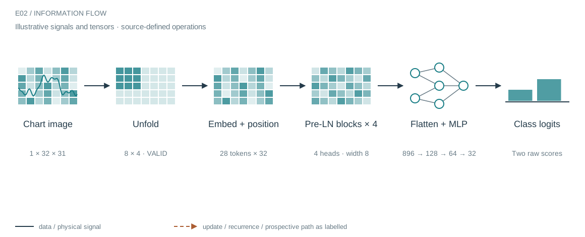
The useful starting point for a framework port is the tensor contract. Here PyTorch receives channels-first images and uses unfold twice. An 8 × 4 stride produces four rows and seven columns of patches: the final three image columns are discarded. That differs from the TensorFlow model’s padded 32-token sequence. This version also uses four transformer blocks and a flattened classification head instead of three blocks and token averaging.
Who does what in the stack
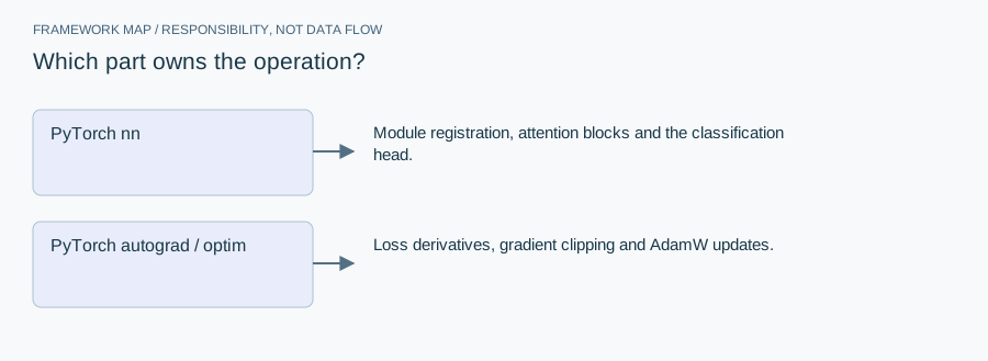
- PyTorch nn
- Module registration, attention blocks and the classification head.
- PyTorch autograd / optim
- Loss derivatives, gradient clipping and AdamW updates.
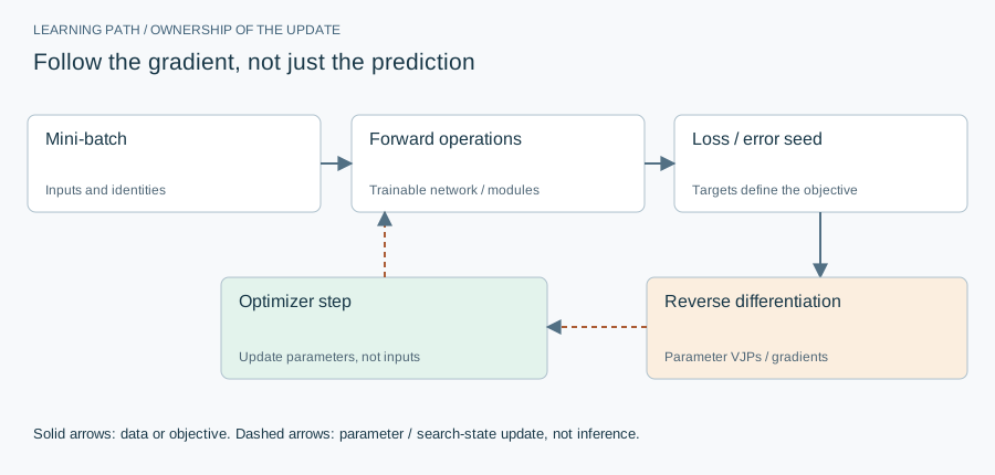
The notebook owns the optimizer loop: AdamW updates follow explicit loss backpropagation, gradient clipping and learning-rate handling. nn.Module owns parameter registration and mode switching; the custom code owns batching, checkpoint decisions and validation. The final training cell is implementation evidence rather than a completed saved training run.
From module map to executable structure
Inside PyTorch patch transformer
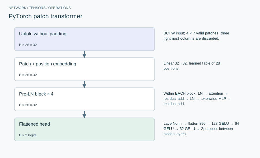
The diagram and count use consistent constructor defaults: image 32 × 31, patch 8 × 4, d=32, 4 heads, 4 blocks. The unexecuted training cell is a different, inconsistent configuration.
| Layer or branch | Output shape | Implementation detail |
|---|---|---|
| Unfold without padding | B × 28 × 32 | BCHW input; 4 × 7 valid patches; three rightmost columns are discarded. |
| Patch + position embedding | B × 28 × 32 | Linear 32→32, learned table of 28 positions. |
| Pre-LN attention × 4 | B × 28 × 32 | LayerNorm → MultiheadAttention(embed_dim=32, heads=4) → residual. Each head has width 8. |
| MLP inside each block | B × 28 × 32 | LayerNorm → 32→64 GELU → dropout → 64→32 → dropout → residual. |
| Flattened head | B × 2 logits | LayerNorm → flatten 896 → 128 GELU → 64 GELU → 32 GELU → 2; dropout between hidden layers. |
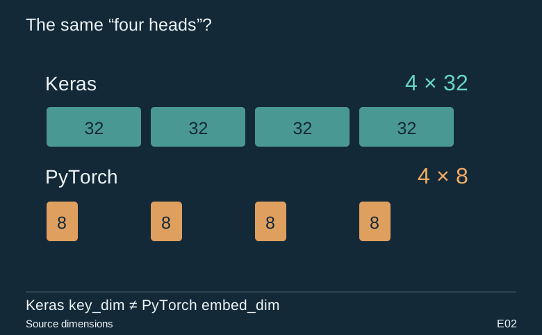
PyTorch divides embed_dim across heads. Setting embed_dim=32 and num_heads=4 therefore produces width 8, not the Keras notebook’s width 32 per head. This changes both parameter count and computation. Flattening all 28 tokens yields 896 head inputs, so the first dense head has 114,816 parameters—larger than all four transformer blocks together. The output remains unnormalized because CrossEntropyLoss performs the log-softmax internally.
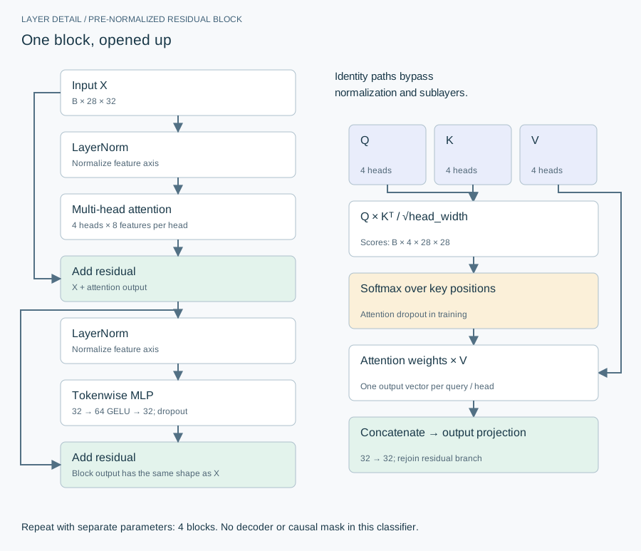
Diagram hierarchy informed by Figures 1–2 of Attention Is All You Need. Original figures here follow the archived classifier code; in particular its pre-LN placement differs from that paper’s post-LN architecture.
The equation and the update
CrossEntropyLoss consumes logits. AdamW: 5e-5 learning rate, 1e-4 decay; batch 256; up to 200 epochs; five-epoch linear warm-up; plateau factor .8 / patience 15; early-stop patience 40; gradient norm clipping at 1.0. The final training cell has no completed execution evidence.
Implementation card / no invented benchmarks
Capacity, budget and execution evidence
- Parameters / retained state
- 161,410 scalars for the default configuration, not the final training-cell configuration.
- Duration and hardware evidence
- MPS-if-available / CPU fallback is coded. No completed timing is claimed for the final training cell.
- Source coordinates
- E02 cell 2, lines 165–272 and 291–365; cells 4–5
- Current reproduction context
- Current workstation, supplied by the author: Apple M4, 128 GB unified RAM, 40 GPU cores and 16 CPU cores. This is context for prospective reproduction, not attribution of every archived run. Python and framework versions are not fully locked for these historical sources; declarations, when available, are identified separately.
Counts above are calculated from the stated layer shapes unless identified as saved measurements. They exclude optimizer state and nontrainable buffers. No archived training was rerun for this revision.
What these design choices change
The final cell selects 25 × 31 images, 5 × 4 patches, embedding 128 and 8 heads. However, PatchEmbedding still calculates position count from hard-coded height 32: 42 positions rather than the actual 35. The first 35 positions can be indexed, but seven embedding rows are unused. Do not describe this as a clean architecture port or reuse the default count for that run. A deliberate repair would pass the image dimensions into PatchEmbedding and test the resulting model as a new version.
Reproduction and measurement protocol
Use the same padded input, embedding widths, block count and pooling strategy before attributing a performance difference to a framework. In this archive those factors are confounded. Check the logits shape and label dtype with a single batch, then test one backward step with dropout disabled. Measure loader time separately: a fast attention kernel will not compensate for serial image decoding.
For a new run, save the resolved Python/framework versions, backend, dtype, seed, input shapes, batch size and exact source revision. Start with one batch and one update. Log training steps separately from epochs or environment steps. Do not equate the configured maximum with a completed budget or convergence.
Measure initialization/compilation, data preparation, warmed forward pass, training updates and evaluation separately. Synchronize accelerator work around timed regions using the chosen framework’s supported mechanism. Report peak process memory and framework allocation separately; parameter bytes exclude activations, gradients, optimizer state and input buffers. On a shared machine, begin with a single CPU worker and a small batch rather than claiming all available resources.
A closer look at the implementation
The code that carries the idea
The two unfold operations expose patch axes without a Python loop over patches. permute places those axes before the patch payload, then reshape produces B × tokens × patch_values. The forward method keeps extraction, embedding, repeated attention and classification separate enough to test individually.
    def extract_patches(self, x):
        B, C, H, W = x.shape
        patches = x.unfold(2, self.patch_height, self.patch_height).\
                   unfold(3, self.patch_width, self.patch_width)
        patches = patches.permute(0, 2, 3, 1, 4, 5)
        patches = patches.reshape(B, -1, C * self.patch_height * self.patch_width)
        return patches

    def forward(self, x):
        # Extract patches
        patches = self.extract_patches(x)

        # Encode patches
        x = self.patch_embedding(patches)

        # Apply transformer blocks
        for block in self.transformer_blocks:
            x = block(x)

        # Classification head
        return self.mlp_head(x)
Verbatim archive excerpt from pt_cnn_transformer_model_lp3_3class.ipynb. Context-dependent historical code, not a standalone runnable program. Comments retain their original wording; the article distinguishes implemented behavior from stale or overbroad comments.
The boundary that matters
PyTorch MultiheadAttention divides embed_dim across its heads. With embed_dim=32 and four heads, each head has eight channels; the Keras example specifies 32 channels per head. Matching the integer “32” in both APIs does not match the attention model.