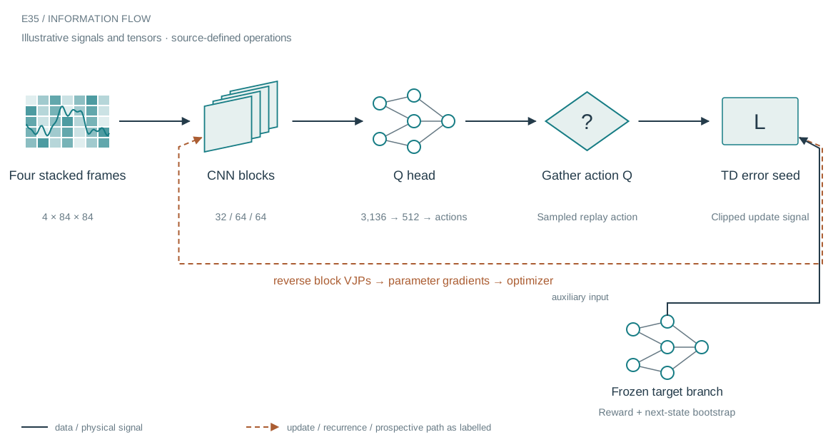
The architecture in context
The system we are building
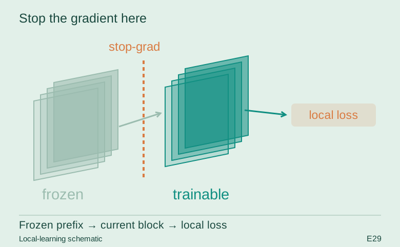
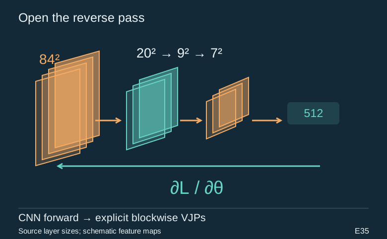
Ordinary loss.backward traverses the connected computation graph. This implementation detaches each block input, records the local input/output pair and later walks those pairs in reverse. The incoming adjoint becomes grad_outputs for a local vector–Jacobian product. In this way the code controls the reverse schedule while PyTorch still computes each block’s derivatives.
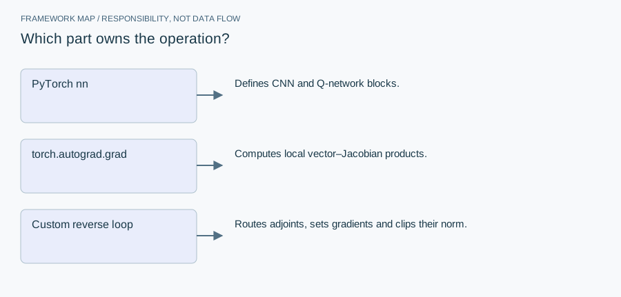
Who does what in the stack
- PyTorch nn
- Defines CNN and Q-network blocks.
- torch.autograd.grad
- Computes local vector–Jacobian products.
- Custom reverse loop
- Routes adjoints, sets gradients and clips their norm.
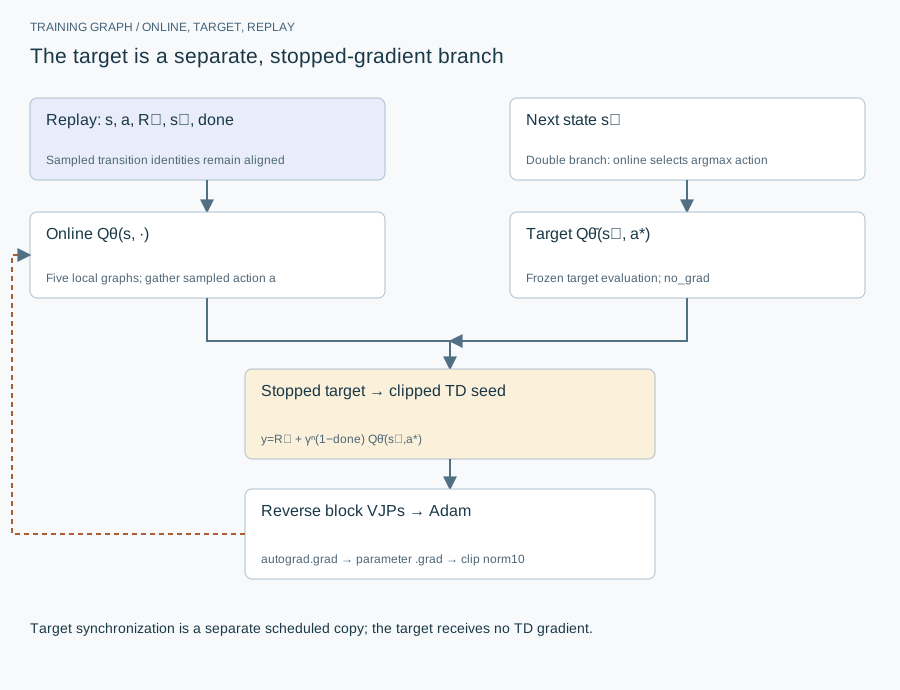
The custom update also constructs DQN or Double-DQN bootstrap targets and seeds an action-specific, clipped TD error. It uses torch.autograd.grad and assigns parameter gradients before the optimizer step. This is different from greedy local contrastive learning: the downstream error still travels through the whole network.
From module map to executable structure
Inside Atari Q-network with explicit reverse VJPs
Stack of four 84×84 grayscale frames; A environment actions; online and target networks.
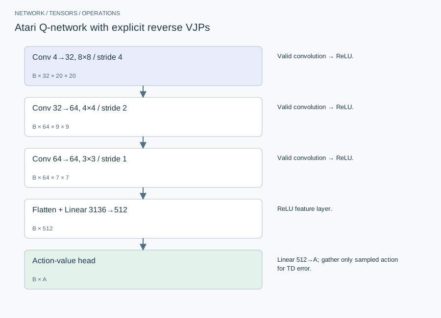
| Layer or branch | Output shape | Implementation detail |
|---|---|---|
| Conv 4→32, 8×8 / stride 4 | B × 32 × 20 × 20 | Valid convolution → ReLU. |
| Conv 32→64, 4×4 / stride 2 | B × 64 × 9 × 9 | Valid convolution → ReLU. |
| Conv 64→64, 3×3 / stride 1 | B × 64 × 7 × 7 | Valid convolution → ReLU. |
| Flatten + Linear 3136→512 | B × 512 | ReLU feature layer. |
| Action-value head | B × A | Linear 512→A; gather only sampled action for TD error. |
The equation shows the Double-DQN branch; the vanilla branch takes the target network’s own maximum. Target construction is under no_grad. Each online block builds a local graph. The reverse loop calls autograd.grad with the next block’s input cotangent, assigns parameter gradients and finally steps Adam. This still implements a reverse chain rule using PyTorch autograd; it is not derivative-free or independent local learning.
The equation and the update
Defaults 400,000 environment steps, replay 50,000, learning starts 10,000, batch 32, Adam 1e-4, gamma .99, target sync 2,000, global gradient-norm cap 10. Smoke overrides:3,000 steps, replay 2,000, start 500, sync 500. Double-DQN and n-step return are selectable flags, not assumptions about every run.
Implementation card / no invented benchmarks
Capacity, budget and execution evidence
- Parameters / retained state
- 1,684,128 + 513A scalars per Q-network; target doubles parameter storage. At A=6:1,687,206 per network.
- Duration and hardware evidence
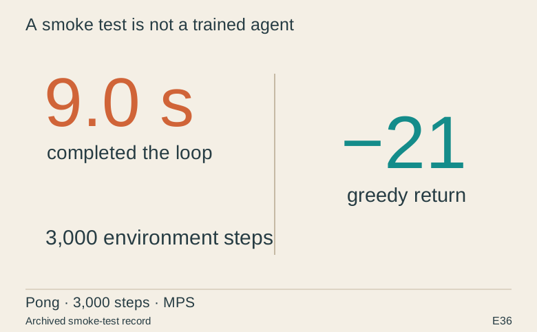
- E36 records a 3,000-step MPS smoke run at 9.0 seconds and final return−21. It does not establish convergence or practical gameplay.
- Source coordinates
- E35 lines 65–108 and 140–160; E36 smoke metrics
- Current reproduction context
- Current workstation, supplied by the author: Apple M4, 128 GB unified RAM, 40 GPU cores and 16 CPU cores. This is context for prospective reproduction, not attribution of every archived run. Python and framework versions are not fully locked for these historical sources; declarations, when available, are identified separately.
Counts above are calculated from the stated layer shapes unless identified as saved measurements. They exclude optimizer state and nontrainable buffers. No archived training was rerun for this revision.
What these design choices change
Strided convolutions reduce the 84×84 image to 7×7 before the large dense layer. That dense layer alone has 1,606,144 parameters, so shrinking it is a materially different capacity choice. Clipping TD residuals and clipping global gradient norm address different instabilities; the factor 2 in the manual seed differs from the usual unit-threshold Huber derivative.
Reproduction and measurement protocol
First compare the manual sweep’s parameter gradients to a monolithic loss with the same scaling, on a fixed tiny replay batch and no optimizer step. Then verify that terminal transitions cannot bootstrap. Count environment steps, replay updates and evaluated episodes separately. A nine-second plumbing test is not a nine-second trained Atari agent.
For a new run, save the resolved Python/framework versions, backend, dtype, seed, input shapes, batch size and exact source revision. Start with one batch and one update. Log training steps separately from epochs or environment steps. Do not equate the configured maximum with a completed budget or convergence.
Measure initialization/compilation, data preparation, warmed forward pass, training updates and evaluation separately. Synchronize accelerator work around timed regions using the chosen framework’s supported mechanism. Report peak process memory and framework allocation separately; parameter bytes exclude activations, gradients, optimizer state and input buffers. On a shared machine, begin with a single CPU worker and a small batch rather than claiming all available resources.
A closer look at the implementation
The code that carries the idea
The essential line requests gradients with respect to both xin and the block parameters. The xin gradient becomes the previous block’s adjoint; parameter gradients are stored for the optimizer. The factor of two and clipping in the seed define this update’s loss scaling, which should be preserved in any equivalence test.
def update(units, target_units, opt, S, A, R, S2, D, gamma, double=False, nstep=1):
    """One (n-step) TD update by the per-block LOCAL sweep -- NO global backward pass. R is the n-step return."""
    with torch.no_grad():
        if double:
            a_star = q_forward(units, S2).argmax(1)                                   # online selects, target evaluates (Double DQN)
            qn = q_forward(target_units, S2).gather(1, a_star[:, None]).squeeze(1)
        else:
            qn = q_forward(target_units, S2).max(1).values                            # vanilla max-Q
        target = R + (gamma ** nstep) * (1 - D) * qn                                  # n-step bootstrap
    x = S; pairs = []
    for u in units:
        xin = x.detach().requires_grad_(True); o = u(xin); pairs.append((u, xin, o)); x = o
    q = x                                                                             # (B, n_act)
    qa = q.gather(1, A[:, None]).squeeze(1)
    diff = (qa - target).clamp(-1, 1)                                                 # Huber-style gradient clip
    d = torch.zeros_like(q); B = len(S); d[torch.arange(B), A] = 2.0 * diff / B       # error only on taken action
    opt.zero_grad()
    for (u, xin, o) in reversed(pairs):
        ps = list(u.parameters()); g = torch.autograd.grad(o, [xin] + ps, grad_outputs=d, allow_unused=True)
        d = g[0]
        for p, gg in zip(ps, g[1:]):
            if gg is not None: p.grad = gg
    torch.nn.utils.clip_grad_norm_([p for u in units for p in u.parameters()], 10.0)  # gradient-norm clip (stability)
    opt.step()
Verbatim archive excerpt from closed_form_neat_dqn_atari.py. Context-dependent historical code, not a standalone runnable program. Comments retain their original wording; the article distinguishes implemented behavior from stale or overbroad comments.
The boundary that matters
Detaching boundaries does not automatically save memory: the code retains local outputs and their graphs until the reverse sweep. Batch normalization, dropout, unused parameters and shared weights require additional care. The saved Pong run is a smoke test, not evidence that this schedule learns a strong policy.