The architecture in context
The system we are building
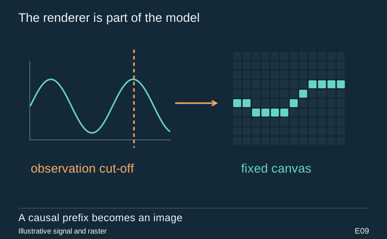
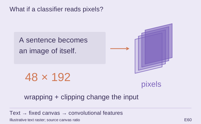
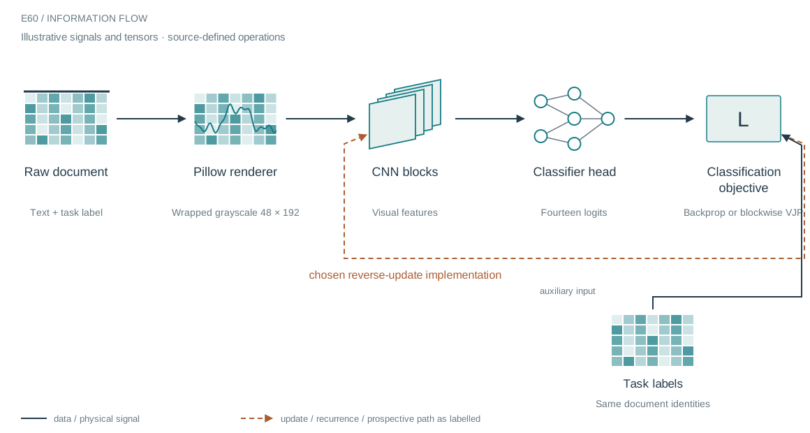
The experiment renders text into fixed-size grayscale images and asks a CNN to predict document categories. This removes the tokenizer from the visual branch but introduces a new front end: font choice, wrapping, raster resolution and clipping. The model sees only the information that survives that renderer.
Who does what in the stack
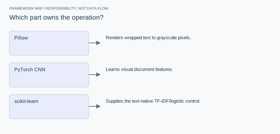
- Pillow
- Renders wrapped text to grayscale pixels.
- PyTorch CNN
- Learns visual document features.
- scikit-learn
- Supplies the text-native TF-IDF/logistic control.
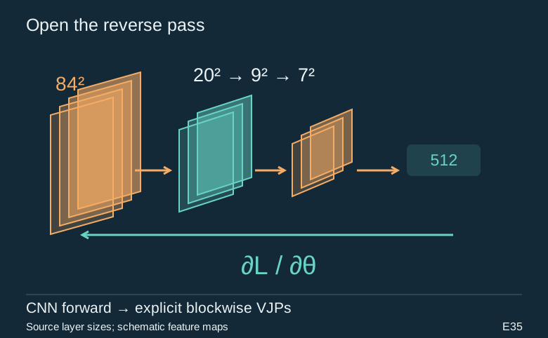
The project adds the text-to-image adapter and a blockwise reverse schedule alongside ordinary backpropagation. The latter still uses PyTorch’s local derivatives; it is not the greedy self-supervised block training in E29. A separate raw-text baseline tests whether the visual representation is useful at all.
From module map to executable structure
Inside Rendered-text convolutional classifier
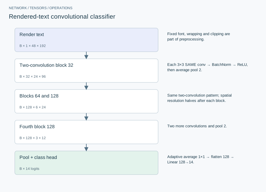
Rendered grayscale 48×192 canvas;14 classes; four blocks of widths 32,64,128,128.
| Layer or branch | Output shape | Implementation detail |
|---|---|---|
| Render text | B × 1 × 48 × 192 | Fixed font, wrapping and clipping are part of preprocessing. |
| Two-convolution block 32 | B × 32 × 24 × 96 | Each 3×3 SAME conv → BatchNorm → ReLU, then average pool 2. |
| Blocks 64 and 128 | B × 128 × 6 × 24 | Same two-convolution pattern; spatial resolution halves after each block. |
| Fourth block 128 | B × 128 × 3 × 12 | Two more convolutions and pool 2. |
| Pool + class head | B × 14 logits | Adaptive average 1×1 → flatten 128 → Linear 128→14. |
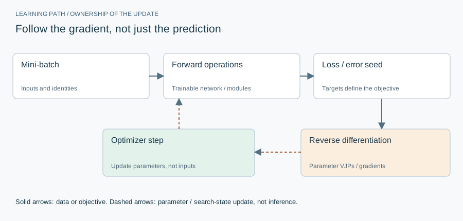
The explicit sweep changes how reverse-mode differentiation is scheduled, not the mathematical supervised objective. It still propagates a global loss gradient backward through every block. This is unlike greedy local contrastive training, which uses independent block losses and freezes preceding modules.
The equation and the update
Adam 2e-3, decay 5e-4, batch 128, cosine learning-rate schedule; configured 30 epochs,2,000 examples per class and two seeds. Compare ordinary backward with an explicit reverse VJP sweep using the same cross-entropy gradient.
Implementation card / no invented benchmarks
Capacity, budget and execution evidence
- Parameters / retained state
- 584,814 scalars, excluding BatchNorm running buffers.
- Duration and hardware evidence
- No elapsed runtime is retained in the selected saved metrics; do not infer training hours from workstation specifications.
- Source coordinates
- E60 lines 20, 58–80 and 91–105; E61 saved metrics
- Current reproduction context
- Current workstation, supplied by the author: Apple M4, 128 GB unified RAM, 40 GPU cores and 16 CPU cores. This is context for prospective reproduction, not attribution of every archived run. Python and framework versions are not fully locked for these historical sources; declarations, when available, are identified separately.
Counts above are calculated from the stated layer shapes unless identified as saved measurements. They exclude optimizer state and nontrainable buffers. No archived training was rerun for this revision.
What these design choices change
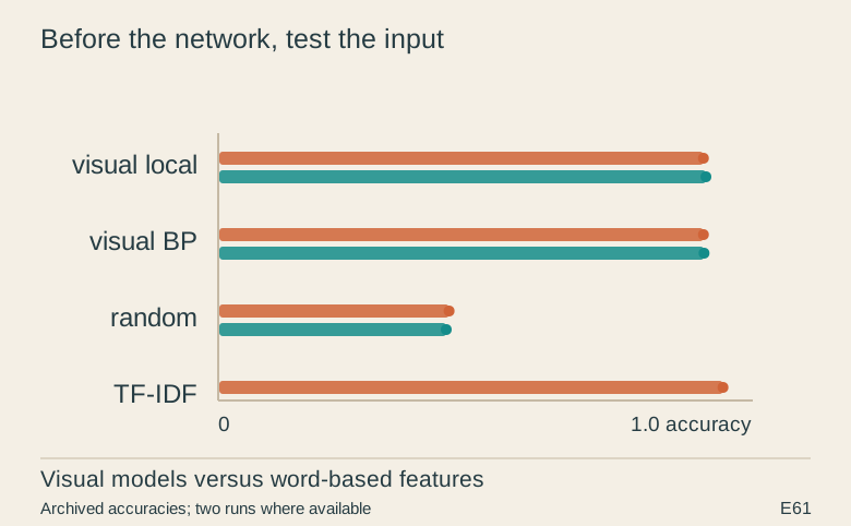
Rendering makes familiar CNN tools applicable but truncates and spatially rearranges text. The TF-IDF control operates on words and word bigrams without paying for a pixel representation. Its stronger saved result is informative: a more elaborate neural input representation is not automatically the better engineering choice.
Reproduction and measurement protocol
Keep a long-text clipping test and a font-availability check next to model tests. Compare gradients before optimizer updates, with identical model state and BatchNorm behavior. Report the word-based logistic-regression baseline as its actual algorithm, not the stale character/ridge description in a comment.
For a new run, save the resolved Python/framework versions, backend, dtype, seed, input shapes, batch size and exact source revision. Start with one batch and one update. Log training steps separately from epochs or environment steps. Do not equate the configured maximum with a completed budget or convergence.
Measure initialization/compilation, data preparation, warmed forward pass, training updates and evaluation separately. Synchronize accelerator work around timed regions using the chosen framework’s supported mechanism. Report peak process memory and framework allocation separately; parameter bytes exclude activations, gradients, optimizer state and input buffers. On a shared machine, begin with a single CPU worker and a small batch rather than claiming all available resources.
A closer look at the implementation
The code that carries the idea
The excerpt wraps text and draws only the lines that fit the canvas. This is an explicit information bottleneck. Two long documents with the same visible prefix can become identical images even if their later content distinguishes their labels.
def render_text(text):
    from PIL import Image, ImageDraw, ImageFont
    font = ImageFont.truetype(FONT_PATH, 10)
    img = Image.new("L", (W, H), 255); d = ImageDraw.Draw(img)
    lines = textwrap.wrap(text, CHARS)[:LINES]
    d.multiline_text((1, 0), "\n".join(lines), font=font, fill=0, spacing=2)
    return np.asarray(img, dtype=np.float32) / 255.0
Verbatim archive excerpt from closed_form_neat_textvision.py. Context-dependent historical code, not a standalone runnable program. Comments retain their original wording; the article distinguishes implemented behavior from stale or overbroad comments.
The boundary that matters
Removing tokenization does not make the model language-agnostic or more efficient end to end. Rendering and image tensors have their own cost. The raw-text comparator receives more directly accessible lexical information; that difference is part of the representation question.