The clock is not always the right unit of work
Imagine an always-on sensor whose internal trace jumps when an event arrives and then decays predictably. A clock-driven implementation keeps revisiting the quiet interval. If the decay is already known, those steps need not discover anything. The interesting question is whether learning can use the entire interval without simulating it one small step at a time.
The learner accumulates time, not snapshots
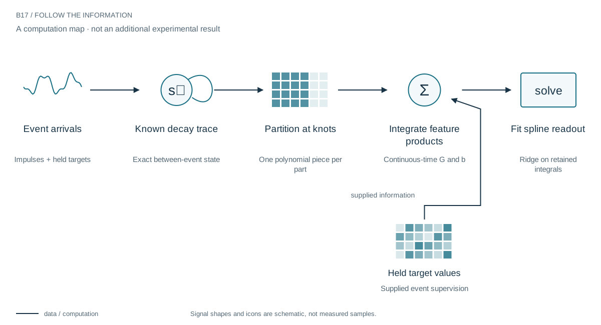
Between impulses, the scalar state follows a known exponential trajectory. A spline readout changes polynomial pieces only when that trajectory crosses a knot. The event routine partitions there and integrates feature products over each interval, so the resulting Gram represents a continuous-time fitting objective. The target is held at its last event value by design.
The quiet tail creates the difficult numerical case. Ordinary time quadrature may spend its nodes poorly, but a comparator that removes the constant contribution analytically resolves the same issue at essentially the same cost. The strongest result is therefore an accurate event-integrated objective, not a speed advantage over every informed alternative.
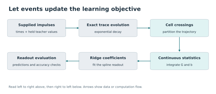
Integrate the learning signal, not just the state
Our readout is a learned spline of the trace amplitude. Within one cell its basis functions are cubic polynomials. As the trace decays through cells, their products can be integrated along the known trajectory. Each interval contributes directly to a Gram matrix and target vector. A later ridge solve uses those statistics rather than replaying a dense synthetic clock.
An assumption that makes the example possible
The experiment supplies event times, the decay constant, and a target held unchanged between events. Those are strong assumptions. We are not recovering an unobserved teacher signal between measurements or training a complete spiking network. The construction asks a cleaner computational question: given this objective, how accurately and cheaply can we accumulate it?
Accuracy was real. The speed headline was not.
Analytic accumulation passes all 48 tested conditions. Several fixed quadrature rules fail on long quiet tails, while midpoint stepping is both inaccurate and slower. But the declared twofold speed advantage over qualified quadrature does not appear. The lesson becomes clearer when we separate the nearly constant part of the final cell: three-point quadrature integrates the remaining polynomial exactly in real arithmetic.
The strong control changes the story
That improved control was constructed after the initial outcomes, so it is an explanatory audit rather than a fresh confirmation. It passes every condition and runs at essentially the same speed as analytic evaluation. The calculus remains useful. What disappears is the claim that one implementation has a distinctive speed advantage merely because its formula is analytic.

An event-driven objective, not yet an event-driven agent
A future event-driven learner could reuse this primitive when both between-event dynamics and supervision semantics are known. Multiple interacting traces, learned events, and delayed rewards need additional machinery. None is supplied by the closed-form scalar integral alone.
What to keep for event-driven ML
The reusable component is a continuous objective accumulated from events under known dynamics. Its value in a larger learner would depend on supervision, state interactions, and the total system cost. No energy or hardware advantage has been measured here. A good event-based algorithm should beat a comparator that understands the same dynamics—not just a clock that unnecessarily ignores them.
Evidence & further reading
The links below distinguish the project record from foundational literature. This revised story does not add a new application-validation experiment.
- Neuromorphic operator learning: mechanisms, evidence and limits. Spline research archive (2026). Local archive snapshot.
- EventProp: exact gradients for spiking neural networks. Timo C. Wunderlich and Christian Pehle (2020). Primary literature.