The model is large. The question is local.
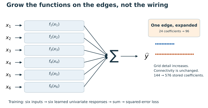
Imagine a learned response curve with 512 coefficients. A particular input does not consult every part of the curve. For a cubic cardinal spline, only four neighboring coefficients influence that prediction. That is an unusually concrete opportunity for a neural-network implementation: much of the representation is irrelevant to the current query. But skipping that work efficiently is a hardware problem as well as a mathematical one.
Inside one forward pass
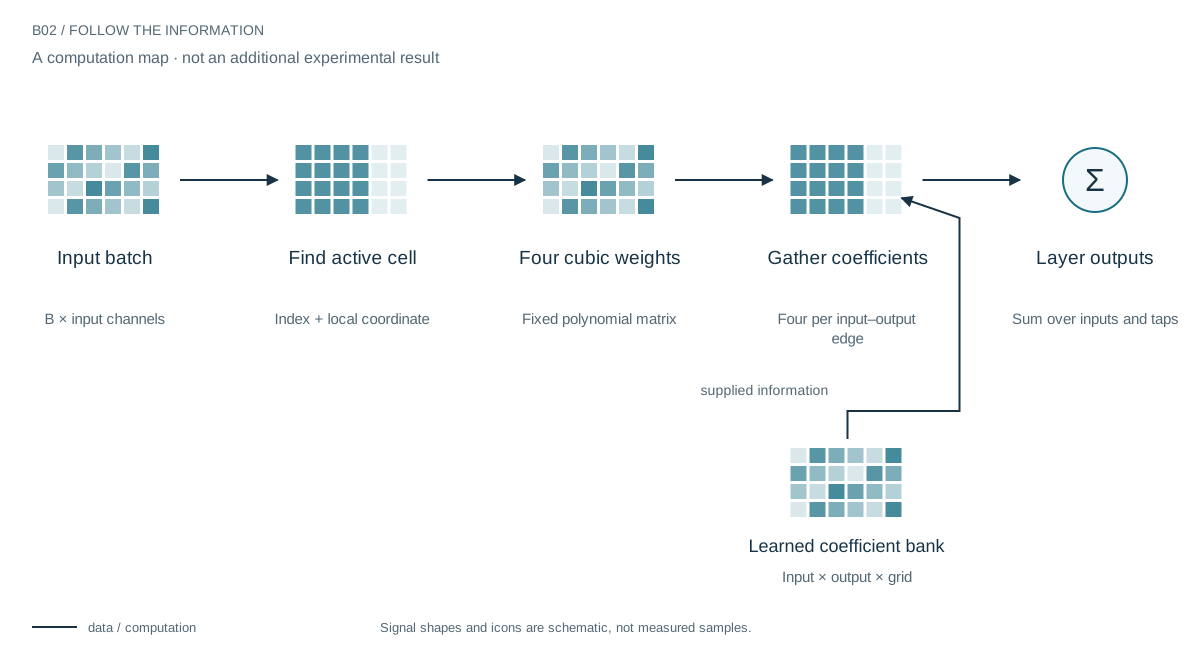
An input batch does not activate an entire grid. For every input channel, the layer finds a cell and computes four weights. Every output channel then reads the four corresponding coefficients of its edge and adds their contributions. The same weight calculation is reused across those outputs. This is where cardinal structure enters the network architecture, rather than remaining an isolated polynomial identity.
The competing dense route first builds a batch-by-input-by-grid feature array. That wastes arithmetic on zeros, but exposes a regular contraction to the accelerator. The local route avoids that array and pays for indexed gathers instead. During coefficient backpropagation, many examples may contribute to the same stored coefficient. A good forward kernel is therefore not automatically a good training kernel.
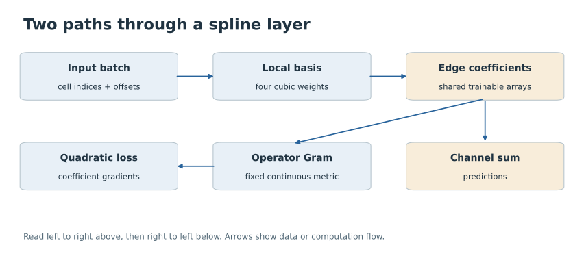
Four weights replace a full basis array
Inside one uniform cell, the four active basis functions are fixed cubic polynomials. A small matrix maps powers of the local coordinate into their weights. The network then gathers the relevant coefficients and sums their contributions. There is no need to run a generic knot recursion for every edge. Nor does the formula require materializing a dense array of mostly zero basis values.
Why the obvious optimization can lose
GPUs are excellent at large regular contractions. A dense basis implementation can exploit that strength, while a local implementation pays for indexed gathers and separate launches. Our streamed implementation processes one of the four taps at a time. This changes the intermediate arrays, but it does not turn every operation into one giant matrix multiplication. Small workloads can favor the ostensibly wasteful dense route.
The crossover is the result
In the archived MPS layer, the batch contains 1024 inputs, with 32 input and 64 output channels. At 512 coefficients per edge, streamed evaluation takes 1.286 ms versus 5.435 ms for dense explicit-cardinal evaluation: 4.23× faster. Including coefficient backpropagation gives 2.95×. At 16, 32, and 64 coefficients, the local route loses. That shape dependence is central to the finding, not a footnote.

Memory needs equally careful accounting
For the largest case, the dense basis array is 64 MiB and one gathered tap is 8 MiB. Those are sizes of particular arrays—not peak process memory or the full training footprint. Coefficients, outputs, temporary buffers, and the backward graph still exist. The benchmark also does not differentiate inputs, so its backward number is not the cost of training a complete deep KAN.
More detail without more work per query
Imagine deploying a fine-resolution learned sensor calibration or control response. The relevant gain is that more grid detail need not increase the number of coefficients touched by one input. Our large-grid measurements demonstrate that opportunity for one layer. Choosing the implementation by workload—and testing input gradients before stacking layers—is the route from that result to an efficient ML component.
A practical route to smaller learned components
The opportunity is a spline component whose implementation follows the active support of its representation. It could matter when high-resolution learned response curves appear repeatedly inside a larger model. A full training-efficiency claim still requires input gradients, peak-memory instrumentation, and end-to-end accuracy at matched work. What is established is useful: local structure has a measured large-grid payoff, and the same measurement tells us when not to use it.
Evidence & further reading
The links below distinguish the project record from foundational literature. This revised story does not add a new application-validation experiment.
- Consolidated research results, including constitutive edges and continual memory. Daniel Schmitter (2026). Local archive snapshot.
- Cardinal Exponential Splines: Part I—Theory and Filtering Algorithms. Michael Unser and Thierry Blu (2005). Primary literature.
- KAN: Kolmogorov–Arnold Networks. Ziming Liu et al. (2024). Primary literature.