What happens between the training points?
A model can fit all observed values and still oscillate between them. A smoothness loss discourages that behavior, but evaluating it at another collection of points creates another sampling problem. For a spline edge with fixed coordinates, the integral itself has an exact finite representation. The model already carries the information needed to compute it.
A loss branch that sees the whole function
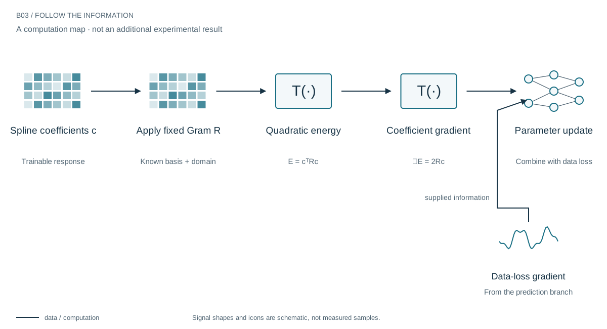
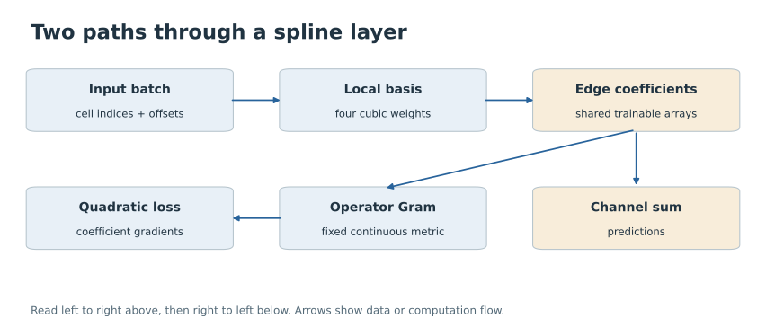
Consider a spline edge inside a learned dynamics model. Its training samples may leave gaps, yet a curvature penalty is meant to control behavior between those samples too. The architecture has a second branch from the coefficient array to a precomputed derivative Gram and then to a scalar energy. It shares parameters with the prediction branch but needs no new sampled inputs.
Backpropagation through this branch is a structured matrix action. For local cubic functions, distant supports do not interact. On a compatible periodic uniform grid, translation invariance provides additional structure. Neither property implies that the empirical data Gram is circulant: its rows depend on where the observations occurred.
Move the integral into the coordinates
Write the curve as a weighted sum of known basis functions. Differentiate those functions, expand the squared derivative, and integrate each pair once. The resulting matrix records how the basis derivatives overlap. Every later loss evaluation is a quadratic form in the current coefficients. Its gradient is a matrix-vector product, without drawing new points to estimate the integral.
Why the matrix is small in practice
Local support means distant basis functions do not overlap, so their inner products are zero. A cubic mass matrix needs only seven neighboring taps on a sufficiently large periodic grid. Uniform spacing and periodic boundaries also make the matrix circulant, allowing Fourier-domain inverse actions. Applying a short stencil can still be cheaper than using an FFT; the right algorithm depends on whether we need a product or a solve.
Exact means exact for the represented function
This calculation measures a specified spline on a specified domain. It does not reveal whether the spline matches an unknown true function. It also does not make an arbitrary empirical neural Gram matrix circulant. Nonuniform weights, changing coordinates, and nonperiodic boundaries can remove that symmetry. If the basis changes during learning, the assembled matrix may no longer describe the intended energy.
What we have actually checked
Archived periodic cubic calculations agree between compact and Fourier implementations near double-precision roundoff. A bounded four-point-per-cell quadrature check agrees with the compact inner product to relative error 2.86 × 10⁻¹⁶. Separately, the grid-growth study finds a modest paired benefit from a continuous curvature penalty on a noisy high-frequency target. We have not measured a universal “10× faster neural loss” result.
Make the loss match the physical function
The practical idea is to stop estimating a known continuous loss anew at every training step. This can make regularization deterministic and tied to physical units. The archive verifies the arithmetic, but does not measure a tenfold end-to-end neural training improvement. A compelling next deployment would measure this loss branch in a real optimization workload, including assembly when the basis changes.
An optimizer should not have to relearn geometry
The broader idea distinguishes a trainable function from its known geometry. Coefficients change; the meaning of a derivative energy need not. That separation can make regularization deterministic, preserve the same penalty when a model grows, and expose efficient linear algebra. It gives ML engineers a precise computational component—not a promise that smoothness always improves generalization.
Evidence & further reading
The links below distinguish the project record from foundational literature. This revised story does not add a new application-validation experiment.
- An Inner-Product Calculus for Periodic Functions and Curves. Anaïs Badoual, Daniel Schmitter and Michael Unser (2016). Primary literature.
- Consolidated research results, including constitutive edges and continual memory. Daniel Schmitter (2026). Local archive snapshot.
- Structure-preservation audit. Spline research archive (2026). Local archive snapshot.
- Operator-spline theory: consolidated research manuscript. Daniel Schmitter (2026). Local archive snapshot.