A model that can make room for detail
A compact learned response often captures broad trends before it can represent narrow features. Increasing capacity should let the model add detail. But an enlarged model is less useful if enlargement itself unexpectedly changes what was already learned.
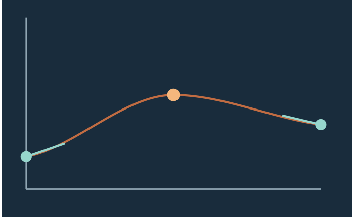
For spline networks, capacity lives partly inside the edges. Each edge is a learned function, represented by basis functions and coefficients. A finer grid provides more local freedom without another input or output. Refinement is therefore an attractive ingredient for adaptive models—and raises a precise question: what should the new coefficients be at the instant of growth?
Our experiment separates three effects: transferring the old function, adding capacity, and learning how to use that capacity.
Here is the network
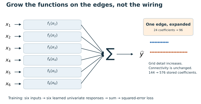
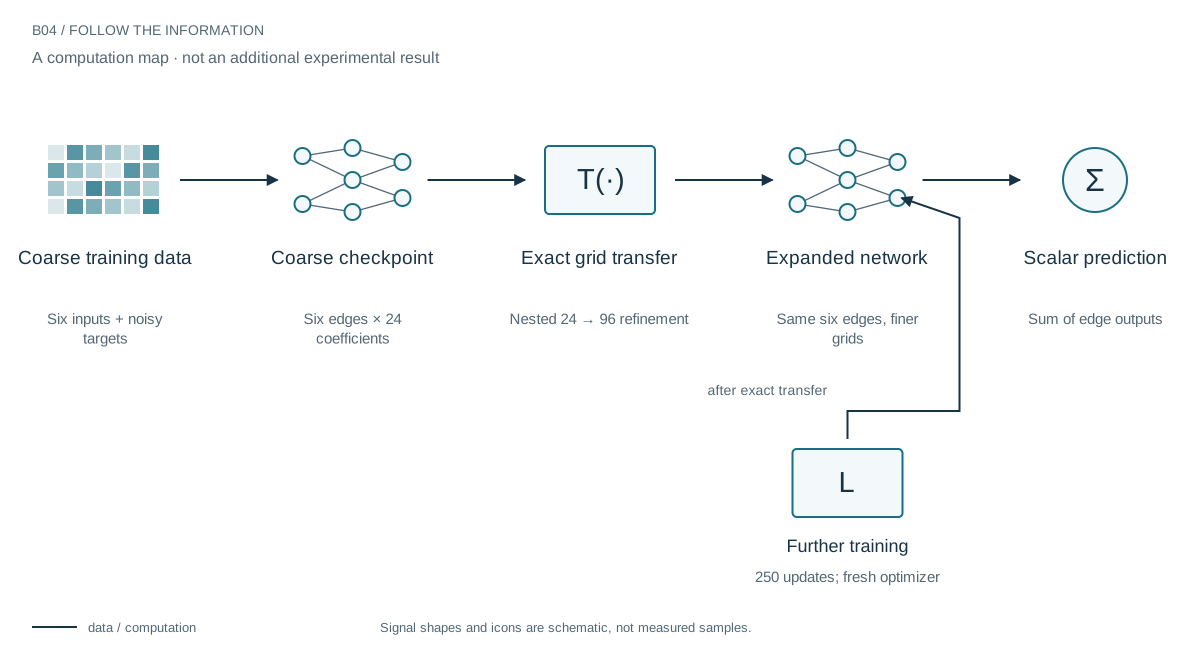
Six scalar inputs feed six spline edges, and a summation node produces one prediction. Each training example supplies a six-dimensional input and a noisy scalar target. The model is not given six separately labeled edge responses.
Each coarse edge stores 24 coefficients: 144 parameters in total. Refinement increases that to 96 per edge, or 576 coefficients, without changing the wiring. Within a cubic edge, one input activates only four neighbors. More coefficients increase resolution across the domain, not the number active at a point.
This is a one-layer additive network, not a deep KAN. It is nonlinear in its inputs but linear in its coefficients. That simplicity isolates grid transfer. Individual edge offsets are not uniquely identified: moving a constant between edges leaves their sum unchanged.
Follow one checkpoint through three operations
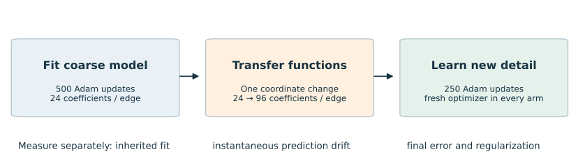
First, train the coarse model for 500 full-batch Adam updates on 4,096 examples. The synthetic target contains broad oscillations, a narrow localized feature, and a high-frequency component. Training labels have 1% noise; 4,096 separate test inputs have clean labels.
Second, expand every edge from the same coarse checkpoint. The arms use continuous projection, coefficient-array interpolation, values at new knots treated as coefficients, or zero restart.
Third, train each arm for 250 further updates with a fresh optimizer. This does not test transfer of Adam moments. We report five paired seeds. The diagram separates an instantaneous representation change from the subsequent learning.
 Open full-size figure ↗
Transfer the function, not the array
Spline coefficients generally are not samples of the represented function. Interpolating their array can change the output even if the new grid looks like a denser version of the old one.
Continuous projection instead asks which function in the new space best approximates the old function over the domain. The cross-Gram matrix measures overlap between the two bases; the new-space Gram matrix converts those overlaps into coefficients. For aligned nested grids, the old function already belongs to the fine space, giving zero approximation error.
For dyadic cubic refinement, a short classical mask performs the same embedding more cheaply than a dense solve. Projection also handles nonnested changes and coarsening. Our independent checks agree with classical refinement and full-rank sampled refitting. Exact preservation is not something existing KAN methods are intrinsically unable to achieve.
What changes at the instant of growth?
Exact transfer changes the trained edge functions by a median relative amount of 1.97 × 10⁻¹⁵: roundoff. Coefficient interpolation changes them by 2.63% and raises immediate test loss by 5.67%. Zero restart discards the inherited function, increasing loss by roughly 71 times.
These are transition results, not final accuracy. They matter when another component immediately consumes a prediction and when a learning comparison should start from the same function. They do not establish a safety guarantee. The values-as-coefficients control even slightly improves median immediate loss while changing the function.
Below, reveal the actual archived test-error checkpoints after expansion. The historical record retained learning curves, not every coefficient state; the animation does not invent those missing states.
Growth is not the end of learning.
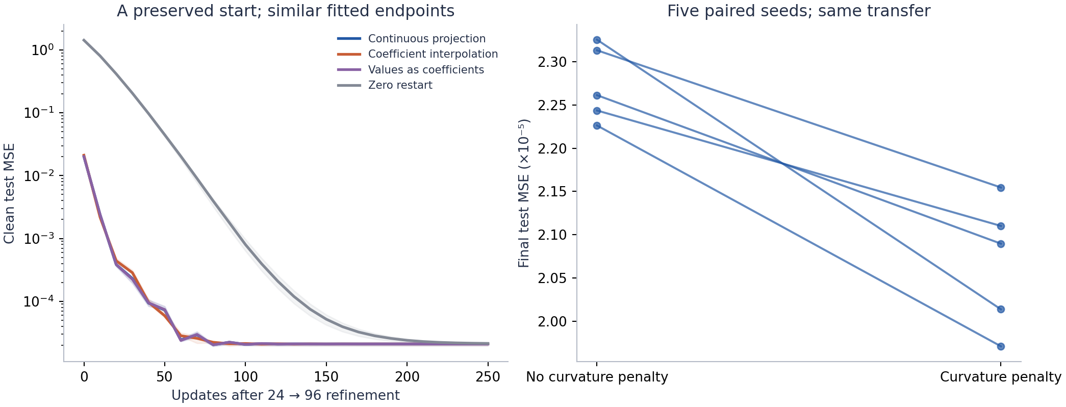
Reveal actual saved test-error curves. All arms have the same fine-grid capacity; their initial functions differ.
New capacity, not a magical initialization
After 250 updates, the three nonzero warm starts reach almost identical test errors. Exact transfer cleans up the transition but does not win the endpoint comparison by itself. That is more useful than selecting a dramatic transient and calling it better learning.
The large improvement comes from giving a deliberately unresolved target enough resolution. Coarse median test MSE is about 0.0201; refinement reaches roughly 2.09 × 10⁻⁵. That change primarily reflects capacity, not the transfer operator.
Continuous curvature regularization gives a smaller independent benefit: median final error falls from 2.26 × 10⁻⁵ to 2.09 × 10⁻⁵, improving all five paired seeds. Integrating the squared curvature measures the represented function, rather than the size of its coefficient array. Its meaning survives an exact refinement.
 Open full-size figure ↗
The experiment where growth was wrong
An earlier smooth target was already fitted well. Exact refinement followed by further training worsened median test error from 5.02 × 10⁻⁶ to 2.24 × 10⁻⁵. The transition itself still preserved the function.
Exact transfer prevents a numerical disturbance; it does not decide whether extra freedom will fit signal or noise. A practical adaptive system needs an independent growth decision and perhaps a way to coarsen. Those decisions remain unvalidated here.
Because this additive model is linear in its coefficients, regularized least squares is also a natural fitting alternative. Adam studies a controlled checkpoint transition; it is not evidence that iterative optimization is necessary or optimal.
A continuous meaning for changing a model
The useful abstraction is a representation change with a specified effect. Nested refinement preserves a function; nonnested transfer gives its best approximation under a declared continuous metric; coarsening trades capacity for quantified error. Continuous regularization measures the same physical quantity before and after refinement.
For this additive architecture, integral-preserving edge projection has another consequence: under independent uniform inputs, integrated squared output disturbance equals the sum of the edge disturbances. The paper derives and numerically checks this relation. Correlated inputs and changing hidden coordinates require different analysis.
The vision is an adaptive model whose resolution can evolve without confusing coordinate changes with learning. We have tested the transition machinery and its limits. A system that decides where and when to grow is the next layer to build.
Evidence & further reading
The companion paper includes the complete protocol, derivation, archived measurements and an independent refinement check.
- Consolidated research results, including constitutive edges and continual memory. Daniel Schmitter (2026). Local archive snapshot.
- An Inner-Product Calculus for Periodic Functions and Curves. Anaïs Badoual, Daniel Schmitter and Michael Unser (2016). Primary literature.
- Operator-spline theory: consolidated research manuscript. Daniel Schmitter (2026). Local archive snapshot.