A boundary is sometimes a fact, not a preference
Imagine learning a short motion that must begin and end at prescribed positions and velocities. A penalty tells the optimizer that violations are expensive. A coordinate construction can make those particular violations impossible within the represented family. The difference is valuable when a constraint is known exactly and should not trade against another objective.
A constrained output layer, not an endpoint penalty
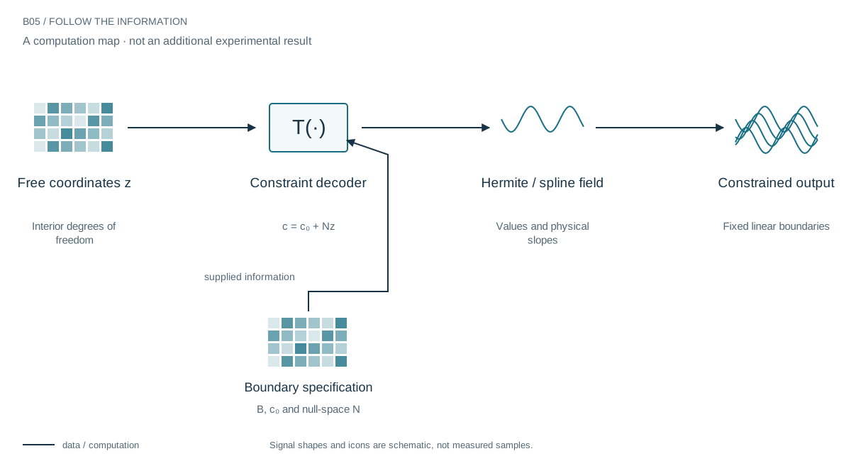
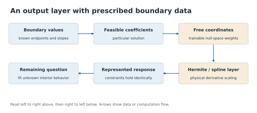
A one-dimensional physical response may need to meet a prescribed value and tangent at each end of an interval. Cubic Hermite coordinates put those four quantities directly in the representation. The derivative coordinates are multiplied by the interval width so that the physical slope does not change when the coordinate is normalized.
For a larger spline component, the same architectural idea writes coefficients as a particular feasible vector plus directions in the null space of the boundary constraints. A network can predict or optimize only those free coordinates. The output layer then maps them into a function that satisfies the linear boundary conditions at every update.
Give the endpoints their own coordinates
A cubic Hermite segment uses its two endpoint values and two endpoint derivatives. Fixing those coordinates enforces the corresponding conditions. A single cubic with all four fixed has no remaining freedom; several connected segments introduce interior degrees of freedom. The animation changes one interior value, not the supposedly fixed endpoints.
The physical units matter
The tangent basis multiplies a physical slope by the cell width. Forgetting that width changes the derivative when the grid changes. This small detail connects geometry to scientific ML: a parameter’s meaning must survive rescaling, refinement, and transfer. Exponential Hermite forms can additionally reproduce supplied dynamical modes, but require their own admissibility and conditioning analysis.
What the construction does not promise
Large tangents do not provide arbitrary resolution inside a coarse cell. Exact endpoints do not prevent overshoot, preserve monotonicity, or satisfy every physical inequality between knots. Those are additional constraints or validation questions. The value of Hermite coordinates is a precise guarantee about a specific boundary—not a universal solution to motion learning.
Choose which facts the learner cannot violate
This is attractive when a boundary is known exactly, such as a clamped displacement or a prescribed endpoint value. It is less appropriate to freeze a noisy measurement as a hard truth. The construction is classical and this article is an explanatory component of the growth paper, not a new benchmark of constrained PINN training. Its value is the explicit separation between facts encoded in an output layer and quantities that remain learnable.
A component for constrained learning
A network can predict the free interior coordinates while a deterministic decoder enforces the known endpoint data. Training then addresses what is unknown. The companion manuscript places this parameterization next to exact refinement and explains which operations preserve the represented function. The guarantee comes from the decoder’s mathematics; an application benefit still needs a task-level experiment.
Evidence & further reading
The links below distinguish the project record from foundational literature. This revised story does not add a new application-validation experiment.
- Operator-spline theory: consolidated research manuscript. Daniel Schmitter (2026). Local archive snapshot.
- Cardinal Exponential Splines: Part I—Theory and Filtering Algorithms. Michael Unser and Thierry Blu (2005). Primary literature.
- Consolidated research results, including constitutive edges and continual memory. Daniel Schmitter (2026). Local archive snapshot.