Put learning where the uncertainty lives
Suppose we know that a field diffuses and that its transport conserves a quantity, but not how flux depends on local state. One approach learns the entire non-diffusive right-hand side. Another learns only that scalar response law and lets a known numerical solver perform the evolution. These are different uses of data—and they lead to different extrapolation mechanisms.
Two ways to spend the same learning effort
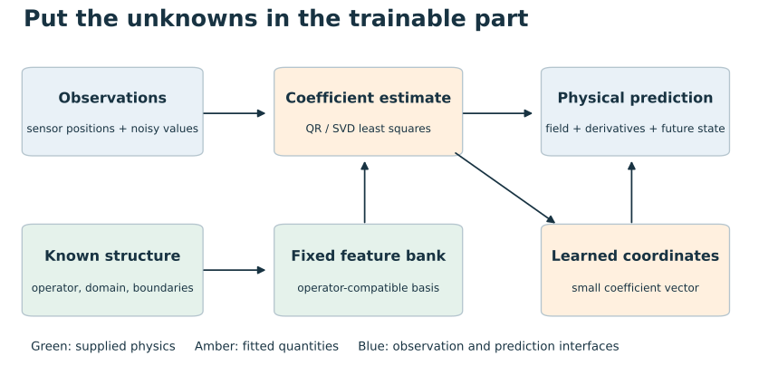
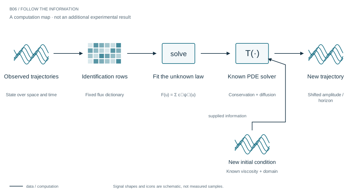
In the structured path, trajectory measurements fit a small scalar law. A known solver supplies conservation, diffusion, and time evolution. In the direct path, a 2–8–1 cardinal KAN or a 2–16–16–1 MLP predicts the non-diffusive state derivative from state and spatial gradient. Both paths still use known viscosity. They are therefore different placements of learning, not a contest in which every architecture receives exactly the same prior.
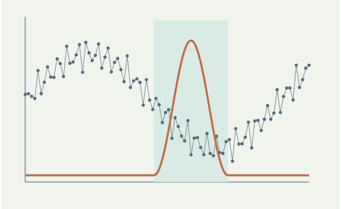
The distinction matters outside the training amplitude range. The learned law can be evaluated inside the same solver at a new state, but its behavior there is determined by its representation. A trigonometric dictionary containing the true oscillation has an unusually favorable continuation. A local spline tail has no corresponding promise.
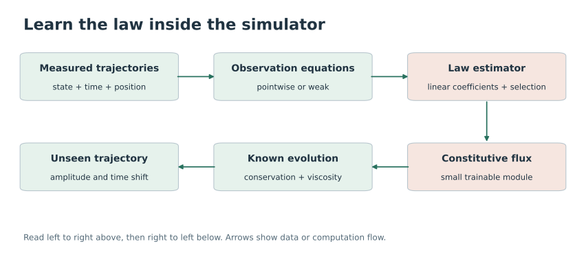
A nonlinear system with a small learnable core
In the equation below, viscosity and the outer derivative structure are given. The unknown function is F. If F is expanded in fixed basis functions, its coefficients enter identification linearly, even though the resulting dynamics remain nonlinear. Learning can become a compact regression rather than a search over every state-to-derivative map. The hard questions shift to excitation, representation, and behavior outside the observed range.
A striking result, with a precise reason
For the synthetic flux one-half u squared plus 0.08 sin(4u), a sparse polynomial–trigonometric library reaches median higher-amplitude, longer-horizon normalized error 9.29 × 10⁻⁷ across three seeds. The direct cardinal KAN control reaches 0.330 and the MLP 0.298. Crucially, the library contains the generating sine component, and the structured model receives the conservation factorization. This is not a pure architecture contest.
The more interesting test is outside the dictionary
A saturating log-cosh flux is not exactly contained in that finite library. The approach reaches median error 0.00520, versus 0.0411 for a structured degree-five polynomial and 0.1165 for the direct MLP. This suggests the representation can help beyond exact component recovery. It remains three deliberately constructed cases, not evidence that arbitrary unknown physics now extrapolates reliably.

Locality is not an extrapolation law
The local spline flux performs much worse under amplitude shift: median error 0.187 for the oscillatory case. Compact support controls where coefficients act, but unobserved tails do not become physically correct by being local. Adding a local residual to an accurate global model can also hurt. Choose a representation for how the unknown law should continue, not only how well it interpolates.
A simulator with a learnable physical core
The larger vision is a simulator that learns a missing material response instead of relearning all of mechanics. The near-exact matched-law result shows what is possible when the interface is right. The unmatched law and failed local tails tell us what still has to be established. That combination is a stronger ML story than a universal claim to beat KAN.
What “beyond a direct KAN” should mean
The experiment supports a more useful question than which network name wins: what must be learned, and what can the model already know? A physics-structured KAN would be a different comparator. The winning dictionary here is not an exponential B-spline kernel. The connection to the operator toolbox is the placement of learning and coherent global components, not a universal spline advantage.
Evidence & further reading
The links below distinguish the project record from foundational literature. This revised story does not add a new application-validation experiment.
- Consolidated research results, including constitutive edges and continual memory. Daniel Schmitter (2026). Local archive snapshot.
- KAN: Kolmogorov–Arnold Networks. Ziming Liu et al. (2024). Primary literature.
- Operator-spline theory: consolidated research manuscript. Daniel Schmitter (2026). Local archive snapshot.