The derivative amplifies the wrong thing
A measured field contains physical variation and observation noise. Subtracting neighboring samples and dividing by a short interval can greatly amplify the latter. If those derivatives become targets, a law learner may explain measurement artifacts. Denser sampling does not automatically solve this; it can make a naive derivative estimate more sensitive. The learning problem begins before the choice of model.
Change the observation layer before changing the network
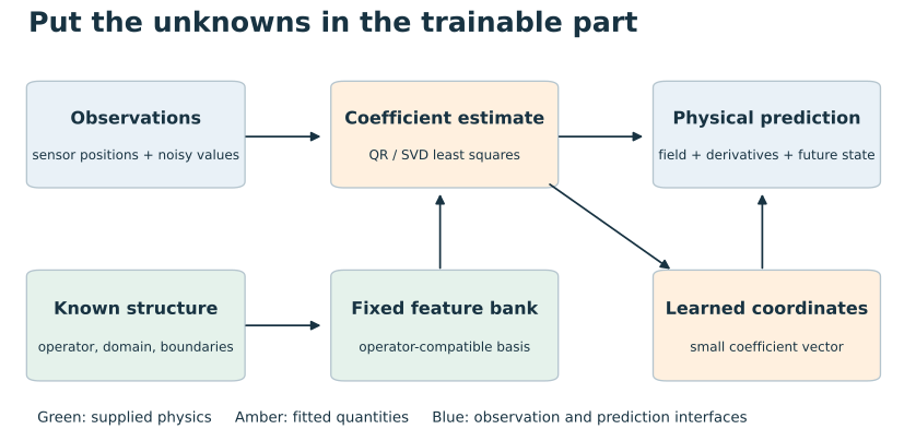
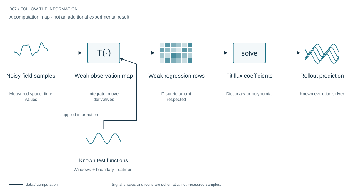
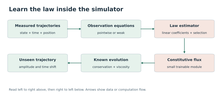
The trainable coefficients need not change when noisy measurements become difficult. What changes is the equation that connects observations to those coefficients. Pointwise fitting estimates time and space derivatives of a noisy trajectory. Weak fitting combines measurements over a window and moves derivatives onto known test functions. Both ultimately feed a small regression system.
The implementation must respect its discrete operators. A sampled continuous test derivative is not necessarily the adjoint of the numerical difference used on the data. The archived construction uses that discrete adjoint explicitly. Its weak rows still overlap in time and space; thousands of rows are not thousands of independent experiments.
Move the derivative to something we control
Multiply the physical equation by a smooth test function and integrate. Integration by parts transfers derivatives from uncertain measurements onto the known test function, with boundary terms handled explicitly. The weak equation asks whether a candidate law explains weighted behavior over a space–time region. This classical principle is used in weak system identification; it is not a new spline invention.
The discrete equation matters too
Our experiment uses compact temporal windows and spatial sine/cosine tests. A subtle detail matters: the temporal operator uses the adjoint of the discrete difference. Sampling a continuous derivative does not necessarily preserve the discrete integration-by-parts identity. Exact calculus is valuable only if the observation model and its numerical implementation describe the same calculation.
A useful improvement, and a useful crossover
At 1% observation noise, median amplitude-shift rollout error falls from 0.03844 for pointwise dictionary fitting to 0.001401 for weak fitting. A weak polynomial gives 0.003194. At 2% noise, the weak dictionary still beats its pointwise counterpart, but the simpler weak polynomial is better: 0.005207 versus 0.006581. Richer representation and better observation handling are different sources of benefit.
Integration is not free information
A test window can suppress noise while hiding fine-scale physics. Its support, boundary behavior, and frequency content determine what is identifiable. Our three-seed synthetic study supplies the outer dynamics and generates controlled noise. It does not reproduce missing variables, irregular sensing, or instrument artifacts from a laboratory. Those uncertainties need their own observation model.
Better evidence before a bigger model
For scientific ML, this suggests an observation layer that expresses trustworthy integral relations before a learned component is fitted. It may improve the information presented to a simple learner more than adding capacity would. The higher-noise polynomial win is important: better observation geometry does not imply that the richest dictionary is the best estimator.
Change the evidence before enlarging the model
A noisy pointwise derivative may be the wrong learning target even for a powerful architecture. The operator view encourages a different representation of evidence: known tests, explicit boundary terms, and coefficient-domain calculations. Splines can support that machinery, but the demonstrated robustness here arises primarily from weak observation formation. The strongest model is not always the best first intervention.
Evidence & further reading
The links below distinguish the project record from foundational literature. This revised story does not add a new application-validation experiment.
- Consolidated research results, including constitutive edges and continual memory. Daniel Schmitter (2026). Local archive snapshot.
- Operator-spline theory: consolidated research manuscript. Daniel Schmitter (2026). Local archive snapshot.