A prediction problem, not an equation on a slide
Imagine a temperature field inside a component. You can measure it at a few locations, but you need the temperature everywhere—and how it will evolve after the next measurement. Or imagine a vibrating structure whose sensors reveal only fragments of its motion. In both cases, fitting a smooth curve through the observations is not the complete task. The model must connect measurements to an unobserved physical state and then produce useful predictions.
Physics-informed neural networks fit observations while penalizing disagreement with a differential equation. But when part of the physics is already known, there is another design choice: put that knowledge into the computation. Which quantities must be learned, and which calculations should never have been a training problem?
Our experiments follow that division of labor from a simple wave to diffusion and an unknown physical law. The opening example introduces the mechanism. The architecture and the progression of experiments explain what we can build with it.
The architecture: fixed physics, learned coordinates
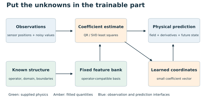
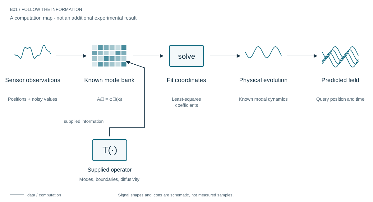
The diagram above is the actual architecture of the fixed-basis examples. Sensor positions enter a known feature bank. Measured values constrain a small coefficient vector. A linear estimator fits those coefficients, and the same feature bank synthesizes predictions between the sensors. For a time-dependent problem, a known evolution operator propagates the fitted state.
In neural-network language, this is a fixed feature layer and a trainable linear readout. The features were chosen to satisfy a physical operator. The learnable coefficients select an admissible solution; they do not teach the feature layer the equation.
Operator-associated spline spaces, local evaluation, and continuous inner products provide ways to construct and manipulate such representations. They do not make every problem linear. Learning operator parameters, latent coordinates, or an unknown nonlinear law leaves additional estimation work.
There are two different computational routes here. A null-space basis makes the encoded equation exact for every coefficient vector. A more general local spline model can instead turn a continuous residual into a quadratic form and solve for its coefficients. That second route removes repeated numerical integration; it does not automatically make the residual zero. If operator parameters are learned, differentiating the linear system gives a compact sensitivity calculation inside a larger learning loop. The paper derives these connections and states which were actually tested.
A wave that obeys the law before fitting
The Helmholtz equation describes spatial patterns associated with a fixed frequency, as arise in wave and vibration problems. In this one-dimensional demonstration, sine and cosine at the supplied frequency both obey the equation. Their amplitudes are unknown. Every amplitude pair describes an admissible candidate—including the wrong pair.
Each sensor contributes one equation in those amplitudes. Fitting 24 observations is a small least-squares problem. The differential equation is satisfied between sensors because of the representation, not because we sampled many residual points.
Below, change measurement noise and sensor placement. The displayed estimate comes from the specified observations and a least-squares calculation. Two modes expose the mechanism; they do not imply that a general physical field has only two unknowns.
Same physics. Different information.
Change the sensors and noise. Both predictions obey the equation, even when the estimate is poor.
Noise reveals what exact physics cannot guarantee
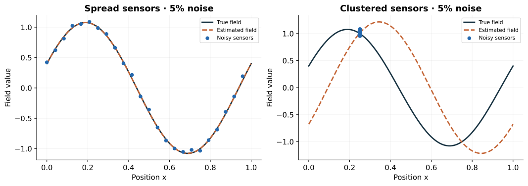
With distributed sensors and 5% noise, median field error is 1.05% across twenty fixed noise realizations. Concentrate the same number of sensors into a narrow region and median error rises to 88.6%. Both fitted fields satisfy the same differential equation. One observation geometry identifies the amplitudes well; the other does not.
This tells us where to invest effort after removing the physics-training loop: sensor placement, excitation, observation modeling, and uncertainty. More accurate calculus cannot replace missing information.
A second failure is representational. Add a higher-frequency component to the true field but keep the two-mode model. Even with noiseless measurements, field error remains 18.3%. An exact residual is an invariant of the model—not proof that its assumptions describe reality.
These are new bounded synthetic studies, with all seeds and definitions in the companion paper. The twenty noise draws are not twenty independent physical systems.
From reconstruction to prediction: heat without retraining
Now consider a rod with zero temperature at both ends, known diffusivity, and an unknown initial temperature profile. Six sine modes satisfy the boundaries. We estimate their amplitudes from 24 noisy initial measurements. Diffusion then determines how quickly each mode decays.
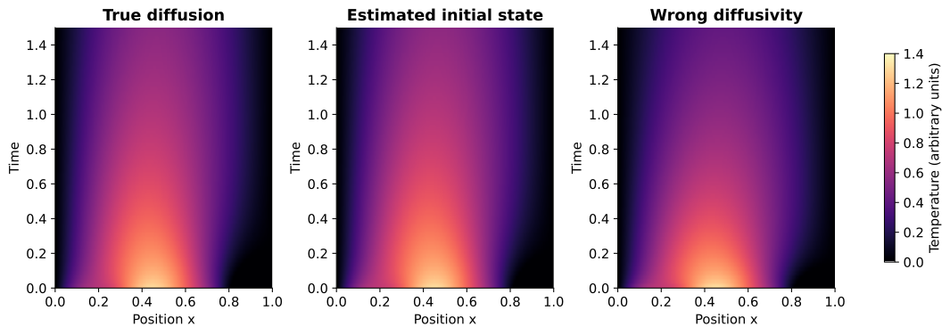
The animation shows the true profile, the reconstructed profile, and the consequence of using the wrong diffusivity. Advancing time does not refit a network: it applies the known evolution to fitted coordinates. The heatmap shows the complete space-time prediction rather than a single attractive frame.
For this fixed example, correct diffusivity gives 2.09% space-time error. Using the same estimated initial state but the wrong diffusivity gives 12.8%. Both models still satisfy the endpoint temperatures. Initial-state estimation and physical-model error are distinct.
The same computational pattern appears in constant-coefficient diffusion, damped dynamics, and the log-price form of constant-volatility Black–Scholes. But boundaries, payoff growth, variable coefficients, and exercise constraints need their own treatment. This heat example is not an options-pricing validation.
Estimate once. Propagate the state.
Orange uses the correct diffusivity. Purple starts identically but evolves under the wrong one.
 Open full-size figure ↗
What our direct PINN comparison actually tells us
The older archive contains a richer field: mixed spatial frequencies on a 128 × 128 periodic grid. A known linear operator produces its forcing. One implementation inverts that operator by Fourier division; another trains a sine-activated coordinate network with data and physics losses.
The CPU record reports field RMSE of 1.97 × 10⁻⁷ for the direct solve in 0.1695 ms, versus 0.212 for the PINN after 109.112 seconds of training. Those numbers explain the original excitement. But the implementation details matter: the direct solver receives full-grid forcing and imposes periodic topology, while the inspected PINN source queries interpolated forcing and has no explicit periodic-boundary enforcement. Several historical run arguments are missing.
We therefore do not present their timing quotient as a universal neural speedup. The FFT path is a classical solver, not a new spline algorithm. The useful lesson survives: first identify the known subproblems that already have reliable direct computations, then compare the remaining learning under matched information.
The deeper opportunity: learn the missing physical law
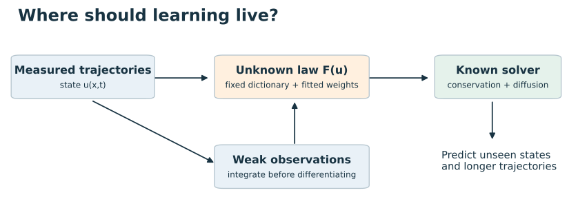
Knowing the complete equation is unusually favorable. A more useful scientific-learning architecture keeps trusted conservation and diffusion structure while learning a constitutive law we do not know. Instead of predicting the entire state derivative with a generic network, a small trainable module predicts the flux F(u); the known solver turns that flux into a trajectory.
Our archived constitutive studies test precisely this placement of learning. They examine amplitude-shift extrapolation and use weak observation equations to reduce noise sensitivity. A dictionary-matched oscillatory law is recovered very accurately; an unmatched saturating law is harder. At the higher reported noise setting, a simpler weak polynomial control beats the richer dictionary.
That is the progression: exact known structure removes avoidable work, informative observations identify what remains, and a learned component extends the system beyond fully specified physics. These are separate experiments, developed in the constitutive article—not additional successes of the two-mode wave model.
 Open full-size figure ↗
What this changes for scientific machine learning
The ambition is a system that assimilates measurements and updates physical predictions without repeatedly relearning established laws. A compact state estimator, a learnable constitutive module, and a structured evolution engine are concrete parts of that system. They need not all use the same representation.
For an ML engineer, this changes the first design question. Does the network need to acquire a representation, identify an unknown law, infer a hidden state, or merely solve for coefficients in a known space? Those are different jobs.
The experiments establish a reproducible part of that vision. The next challenge is not another perfect residual on a matched example. It is accurate prediction when the operator, observations, and representation are only partially right. That is where the architecture—not just the equation—earns its place.
Evidence & further reading
The dedicated companion paper includes the new synthetic sensor and heat studies, all numerical definitions, and an audit of the separate historical comparison.
- Operator-spline theory: consolidated research manuscript. Daniel Schmitter (2026). Local archive snapshot.
- Consolidated research results, including constitutive edges and continual memory. Daniel Schmitter (2026). Local archive snapshot.
- Physics-informed neural networks: A deep learning framework for solving forward and inverse problems involving nonlinear partial differential equations. Maziar Raissi, Paris Perdikaris and George Em Karniadakis (2019). Primary literature.
- Cardinal Exponential Splines: Part I—Theory and Filtering Algorithms. Michael Unser and Thierry Blu (2005). Primary literature.