Physics is a guide, not a substitute for the task
A velocity field should satisfy appropriate physical laws. Enforcing one law can improve reconstruction, but an application may ask where a particle will travel rather than how small a global residual becomes. The particle repeatedly samples particular regions. A globally improved field can still be worse along its path.
One correction, three possible objectives
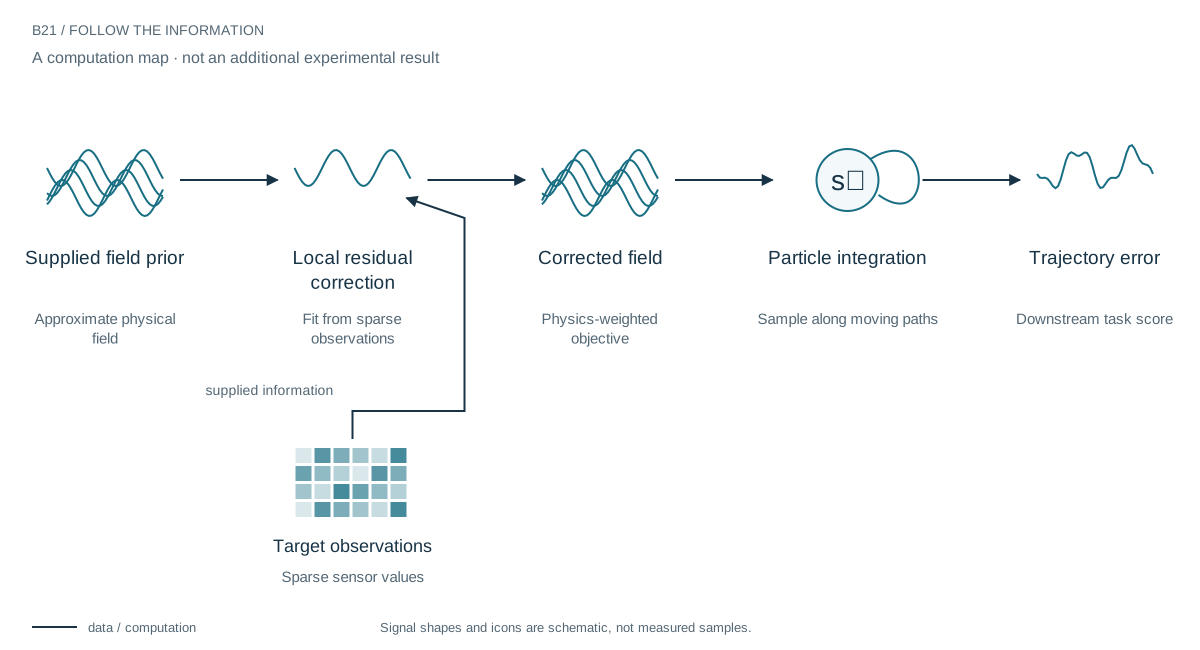
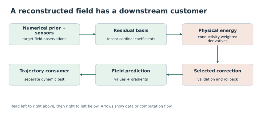
The Darcy model begins with a supplied finite-volume prior and 32 observed solution values. A small cardinal residual adjusts the field, while conductivity-weighted derivative energy prefers certain corrections. A few sensors select a strength or rollback before refitting. This is per-field assimilation with target observations, not forecasting an unseen solution from its coefficients alone.
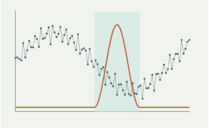
The turbulence extension asks a different question: where do particles go? They repeatedly sample a changing path through the approximate velocity. A global field norm and a divergence penalty do not control all errors encountered on that path. The observed all-frame field improvement and all-stream trajectory deterioration expose that mismatch.
A positive result with a matched ablation
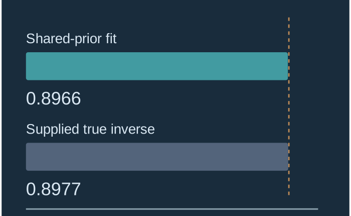
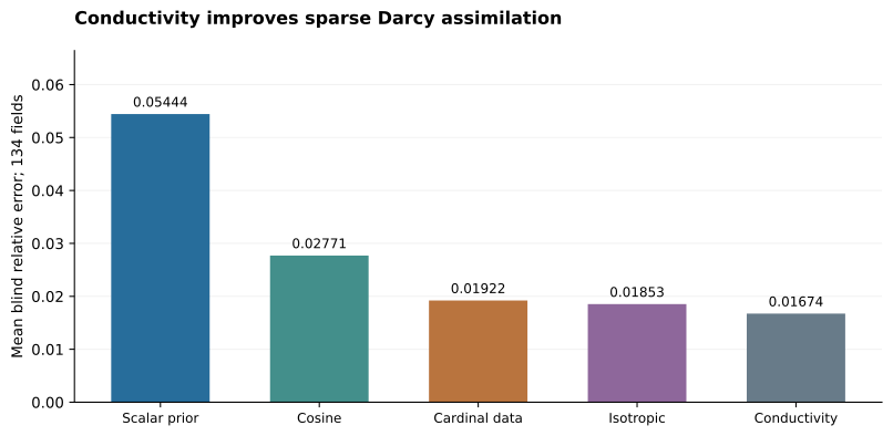
On 134 Darcy confirmation fields, a cardinal correction using known conductivity and 32 observed solution values reduces mean blind error from 0.02771 for a selected cosine residual to 0.01674. Removing conductivity weighting from the same basis worsens the result. This is sparse target-field assimilation, not forecasting without observations. A discrete strong-form mismatch actually becomes worse.
The dynamic test reversed the conclusion
The turbulence follow-up freezes a divergence-informed correction and tests six new five-frame streams. Blind velocity error improves on all thirty frames. Yet endpoint and all-time particle errors worsen on all six streams, with paired median deteriorations of 7.34% and 6.56%. The simpler uncorrected interpolation is the relevant control; beating a slower PINN alternative would not erase this failure.
Why the mathematics allows it
Trajectory stability depends on velocity error where the trajectories go, together with the field’s sensitivity to position. A global mean-square norm does not automatically bound that error. Nor does divergence determine velocity: even a constant added drift preserves divergence but changes a path. The physical penalty addresses one property, not the entire prediction problem.
Train for the quantity the application consumes
The scientific opportunity is a learned correction whose metric reflects the quantity an application consumes. A field visualization, a flux estimate, and a trajectory forecast may need different loss functions. The toolbox makes these quantities easier to express; it does not select the right one on behalf of the application.
Choose the learned object around its use
If the application consumes a flow map, an experiment should score that flow map directly. If it consumes a field or an energy, those are legitimate objectives too. The operator toolbox makes such quantities computable; it does not decide which one matters. This positive-and-negative pair is a concrete reason to connect the mathematical objective to the downstream scientific question.
Evidence & further reading
The links below distinguish the project record from foundational literature. This revised story does not add a new application-validation experiment.
- Consolidated research results, including constitutive edges and continual memory. Daniel Schmitter (2026). Local archive snapshot.
- Consolidated limitations and research boundaries. Daniel Schmitter (2026). Local archive snapshot.
- Experiment-family evidence map. Spline research archive (2026). Local archive snapshot.
- Physics-informed neural networks: A deep learning framework for solving forward and inverse problems involving nonlinear partial differential equations. Maziar Raissi, Paris Perdikaris and George Em Karniadakis (2019). Primary literature.