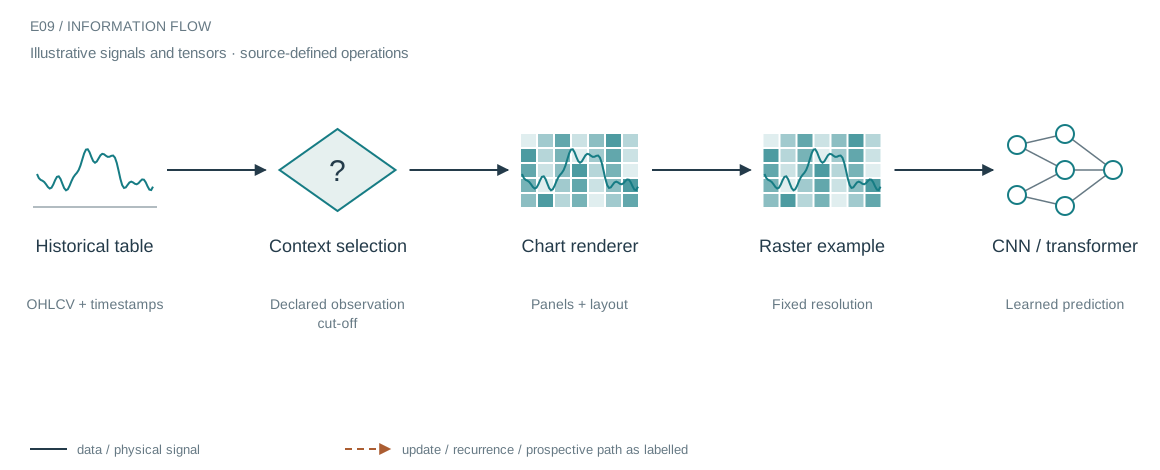
The architecture in context
The system we are building
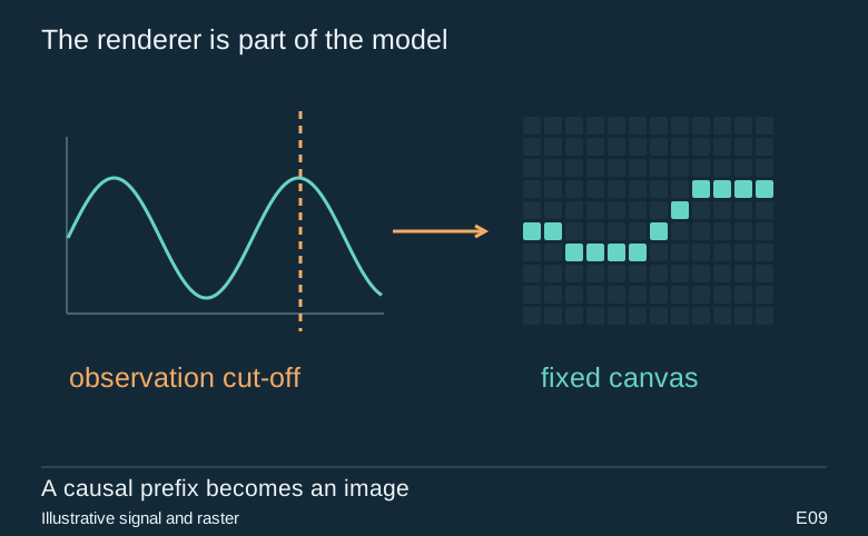
This module creates structured chart images rather than photographing a screen. It selects historical sessions, builds OHLC and volume tables, adds contextual panels and saves an image with identifiers in its filename. The renderer is a feature transform: line widths, scaling, panel arrangement and image resolution determine what the neural model can observe.
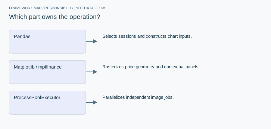
Who does what in the stack
- Pandas
- Selects sessions and constructs chart inputs.
- Matplotlib / mplfinance
- Rasterizes price geometry and contextual panels.
- ProcessPoolExecutor
- Parallelizes independent image jobs.
Several figure builders explore different visual representations over the same underlying data. Multiprocessing is used around image creation, while Matplotlib and mplfinance handle drawing. That separation lets representation experiments reuse a classifier without pretending that the input distribution stayed unchanged.
Open up the implementation
Make the observation clock part of the image
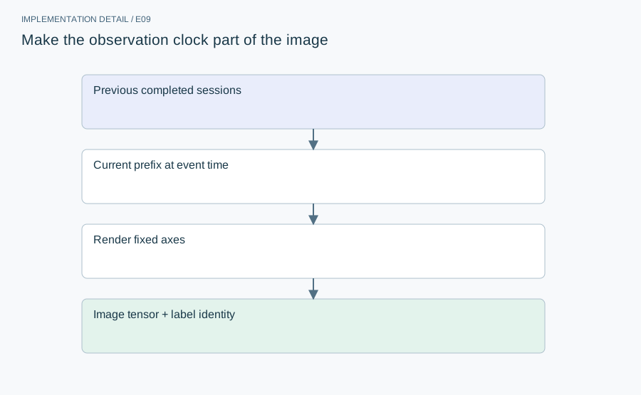
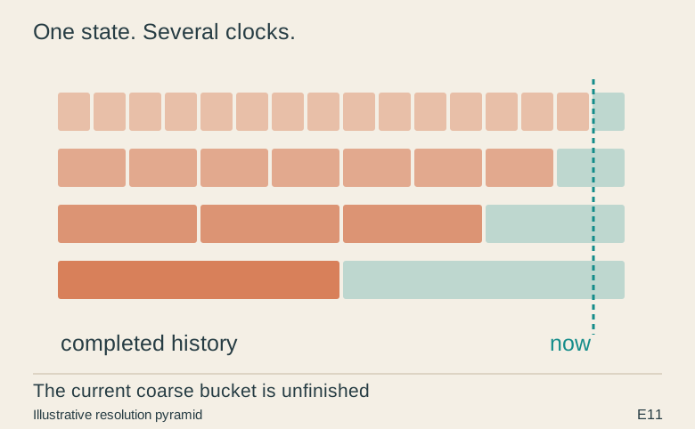
The image is a learned model’s representation of a time series. This implementation includes complete prior sessions and a current-session prefix up to the adjusted observation time. The causal claim belongs to which values were available at that time, not the date printed on the chart. A renderer that rescales axes using a later full-day range can leak future context even if it plots only the prefix.
The mathematical contract
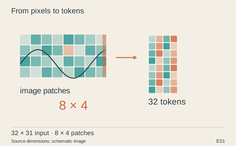
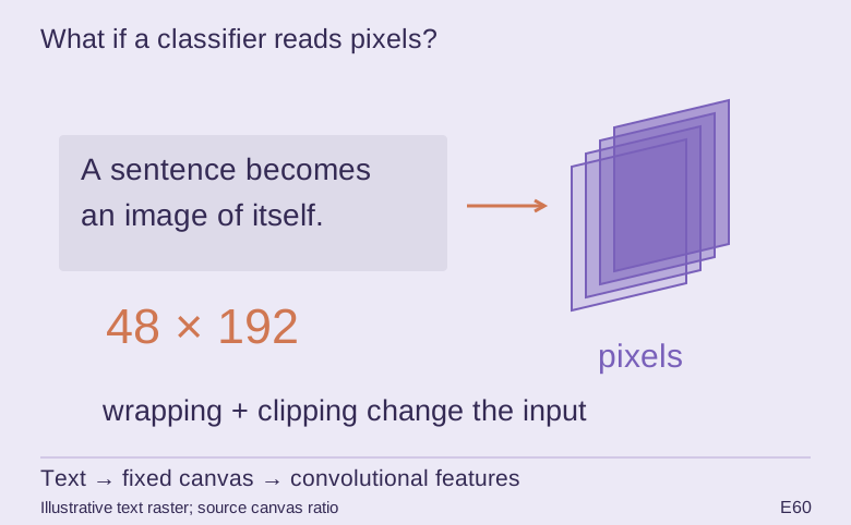
Rendering enables reuse of CNNs but introduces choices about pixel resolution, line thickness, cropping and axes. Those choices alter the signal seen by patch extraction. They must remain stable between training and inference, or the apparent architecture comparison becomes a preprocessing comparison.
Implementation and resource card
- Capacity / budget
- No trainable layers in the renderer. Canvas dimensions, color normalization and cut-off time are model input hyperparameters.
- Execution evidence
- This revision inspects and explains the archived implementation. It does not rerun the original workload. No unrecorded convergence time, throughput or accelerator result is supplied.
- Current reproduction context
- Current workstation, supplied by the author: Apple M4, 128 GB unified RAM, 40 GPU cores and 16 CPU cores. This is context for prospective reproduction, not attribution of every archived run. Python and framework versions are not fully locked for these historical sources; declarations, when available, are identified separately.
From explanation to a reproducible check
Create two series identical before a cut-off and radically different afterward. Their rendered input at the cut-off should match under a causal pipeline. Check price-axis limits, volume normalization, captions and filenames as well as the plotted line.
Preserve input identities, configuration and failure records with the result. A successful numerical check only establishes the operation it exercises: it does not certify an entire dataset, model or deployed system. Reproduce the interface on a small deterministic input before optimizing throughput or increasing workload size.
A closer look at the implementation
The code that carries the idea
The selected function uses complete prior sessions but cuts the current day at adjusted_Open_time. It then concatenates three prior dates with the partial current session. The cutoff is a local indexing choice, not a complete proof of causality: the availability of each panel’s source values still needs to be reconciled with the prediction timestamp.
def create_time_series_us_tickers(dates_array, dataframe: pd.DataFrame):
    # Ensure 'Time' column is of type datetime.time only if it's currently of type str
    if isinstance(dataframe['Time'].iloc[0], str):
        dataframe['Time'] = dataframe['Time'].apply(lambda x: datetime.strptime(x, '%H:%M:%S').time())

    # Filter the dataframe to capture data up to the European market closing time (11:30:00 EDT = UTC 16:30:00 or 17:30:00)
    # FIXME: ensure opening times are correct and adjust them to 11:50 (due to 20' delay in receiving EUR-ticker data)
    # filtered_data = dataframe[dataframe['Time'] < dataframe['adjusted_Open_time']] # DE-BUG: not proper: takes first timestamp of the day, which is pre-market opening time
    adjusted_data_today = dataframe[(dataframe['Time'] <= dataframe['adjusted_Open_time']) & (dataframe['Time'] >= dataframe['nyse_nasdaq_open_time'])]
    adjusted_data_prev_days = dataframe[(dataframe['Time'] >= dataframe['nyse_nasdaq_open_time']) & (dataframe['Time'] <= dataframe['nyse_nasdaq_close_time'])]

    full_data_today = dataframe[(dataframe['Time'] <= dataframe['adjusted_Open_time'])]
    full_data_prev_days = dataframe

    # Get the date n days back
    date_today = dates_array[-1]
    date_previous_day1 = dates_array[-2] #get_date_n_days_back(dataframe, date_today, 1)
    date_previous_day2 = dates_array[-3] #get_date_n_days_back(dataframe, date_today, 2)
    date_previous_day3 = dates_array[-4] #get_date_n_days_back(dataframe, date_today, 3)

    four_day_time_series_adjusted_data = pd.concat([adjusted_data_prev_days[adjusted_data_prev_days['Date'] == date_previous_day3],
                                                    adjusted_data_prev_days[adjusted_data_prev_days['Date'] == date_previous_day2],
Verbatim archive excerpt from cnn_image_functions.py. Context-dependent historical code, not a standalone runnable program. Comments retain their original wording; the article distinguishes implemented behavior from stale or overbroad comments.
The boundary that matters
Images can hide leakage more effectively than numeric tables. A globally chosen vertical scale, an end-of-session volume statistic or a future-derived annotation can all enter as pixels. A model may also learn plot artifacts instead of the intended geometry.