Start by following the error
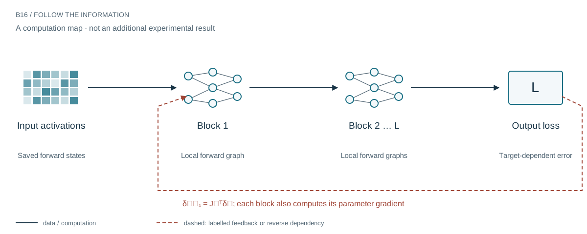
Suppose a network is trained one block at a time, each with its own local automatic-differentiation graph. That sounds unlike a global backward pass. But if each block receives an output error, multiplies it by its transposed Jacobian, and passes the result to the preceding block, the computation is still reverse-mode differentiation. The software packaging changed; the chain rule did not.
Draw the arrows before naming the learning rule
The blockwise implementation explicitly passes the loss derivative backward from one local graph to the previous one. Detaching the forward activations does not remove that information path. Under fixed forward states, the resulting parameter gradients are the chain rule. The new diagram therefore shows both the forward activation path and the reverse credit dependency.
The relaxation alternative is different: hidden values move iteratively while weights are fixed, then local energy derivatives update the weights. Fifteen iterations provide excellent alignment near the output but poor alignment near the input in the retained diagnostic. A good last-layer match cannot represent the whole network.
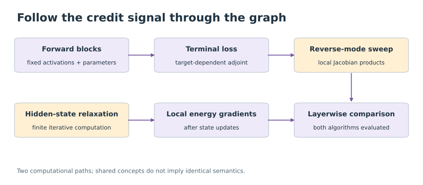
Our exact sweep is backpropagation
Source inspection shows precisely this mechanism in the archived blockwise vision runner. A bounded test extracts its actual update functions and compares them with a global backward pass on small deterministic networks. Across three seeds, binary64 gradients agree within about 3.6 × 10⁻¹⁶ relative error. Separate finite differences check their scale. This is an implementation identity, not a discovery that gradients can be avoided.
The vision comparison fits that interpretation
In the named two-seed CIFAR-100 panel, global and blockwise means are 69.16% and 69.05%. The paired difference changes sign between seeds. We retain both outcomes. If mathematically identical derivatives produce different long training trajectories, the explanation must involve execution, numerical effects, randomness, or changed conditions—not an intrinsic new learning principle.
Predictive-coding relaxation asks a different question
A separate implementation repeatedly adjusts hidden states to reduce adjacent-layer prediction errors, then updates weights. Its result depends on how long it settles, the nudge, and the step size. It is not the exact one-pass recurrence under another name. The retained convolutional run reaches 39.93% accuracy versus 54.47% for its squared-error backpropagation control.
Look at every layer, not only the last
The alignment diagnostic explains why output-side agreement can be misleading. At fifteen relaxation steps, the last blocks closely match the reference direction, while the first blocks do not. Even the longest tested setting leaves the first cosine at 0.0805. Cosine alone also misses magnitude differences. The figure shows every configuration and block rather than a selected near-one value.

Measure locality as an engineering property
Local computation remains a worthwhile systems direction. It may enable scheduling, modularity, or specialized hardware. The research becomes stronger when those benefits are measured separately from a claim to have invented a different gradient. Here the exact-gradient result and the finite-relaxation failure are both retained.
Local computation is still worth studying
Modular reverse-mode execution may offer engineering advantages, and genuinely different local dynamics may offer useful tradeoffs. Both deserve precise measurements. What does not help is assigning a biological or gradient-free interpretation before identifying the computation. The strongest story here is an explicit distinction that makes the next learning experiment scientifically testable.
Evidence & further reading
The links below distinguish the project record from foundational literature. This revised story does not add a new application-validation experiment.
- Consolidated research results, including constitutive edges and continual memory. Daniel Schmitter (2026). Local archive snapshot.
- Full experimental record. Daniel Schmitter (2026). Local archive snapshot.
- Negative-result appendix. Daniel Schmitter (2026). Local archive snapshot.
- Operator-spline theory: consolidated research manuscript. Daniel Schmitter (2026). Local archive snapshot.