Two problems hide inside one search
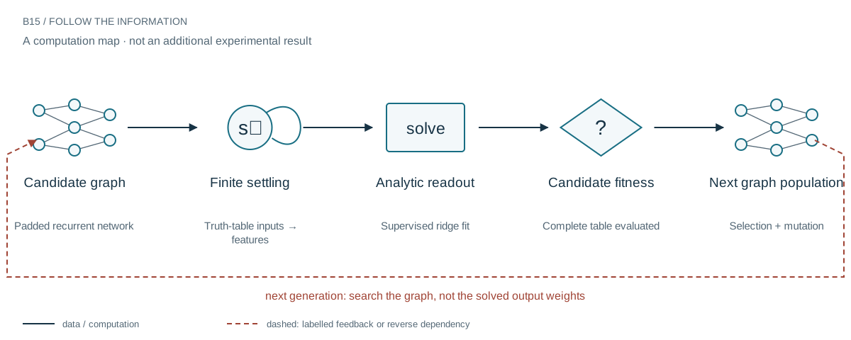
A candidate network has to generate useful features and turn those features into an answer. In a supervised quadratic problem, the second task has a direct regularized solution once the first is fixed. We let evolution change a small recurrent graph while a ridge solve fits its readout. That is a concrete allocation of work—not a claim that evolution or matrix inversion becomes free.
An evolutionary loop with an exact inner problem
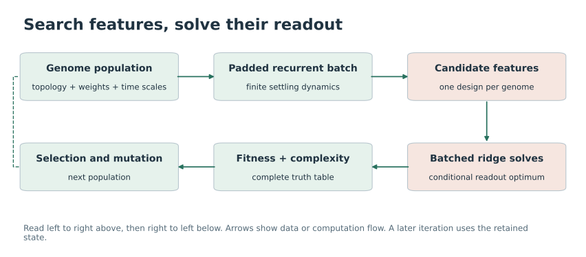
A candidate graph is first converted into a padded recurrent feature computation. It settles for a fixed number of steps, producing features for every supplied truth-table input. A batched ridge solve chooses its supervised readout. Evolution then evaluates that fitted candidate and changes the nonlinear graph.
This division removes output-weight search conditional on the candidate features. It does not remove architecture search, make finite settling an equilibrium solve, or supply targets in reinforcement learning. The distinction between padding and mutation also matters: an inactive zero feature preserves predictions, but a new nonlinear leaky node generally does not.
Make irregular candidates compatible with regular hardware
The implementation maps each graph into padded arrays, zeros its inactive coordinates, and evaluates a population with batched matrix operations. Different topologies then share a computational shape without becoming the same graph. Zero padding preserves the ridge prediction; cutting off active nodes at a capacity limit does not. Dense padding also costs memory and arithmetic, even where most connections are absent.
What the finite construction study accomplished
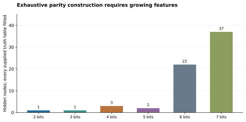
The named sweep fits complete parity truth tables from two through seven input bits. Seven-bit parity uses 37 hidden units and 119 generations; the recorded sweep takes 36.3 seconds for that rung. Every truth-table row participates in fitting and selection, so this is construction of a finite function, not generalization to unseen parity examples or longer sequences.
Growth has more than one meaning
Splitting a connection through a tanh unit is only approximately an identity in a limited amplitude range. The new leaky state also adds a transient. It therefore does not inherit the exact preservation guarantee of nested spline refinement. A small diagnostic makes the static discrepancy visible even when the outgoing weight compensates the incoming scale.
The comparator needs the same question
Canonical NEAT does not require an inner backpropagation loop. The saved neat-python reference differs in activation, recurrence, readout, input scaling, fitness, population, and hardware execution. Its failure on several rungs cannot isolate the analytic readout’s benefit. We report the construction results without turning this unmatched comparison into an orders-of-magnitude speed claim.
Use search only where a solve is unavailable
The broader pattern is to reserve expensive search for variables that genuinely need it. Parity through seven bits is a finite construction demonstration of that pattern. A convincing new application would need held-out behavior and matched outer-search controls, rather than treating one unmatched NEAT timing as a universal result.
A reusable pattern, with a clear boundary
Search over structure; solve the conditionally linear part. That pattern connects this experiment to classical variable projection and operator-based models. It is useful when supervised targets and a quadratic inner objective exist. If an agent receives only delayed reward, the targets needed by the solve do not appear automatically. The research question then changes.
Evidence & further reading
The links below distinguish the project record from foundational literature. This revised story does not add a new application-validation experiment.
- Evolving Neural Networks through Augmenting Topologies. Kenneth O. Stanley and Risto Miikkulainen (2002). Primary literature.
- Consolidated research results, including constitutive edges and continual memory. Daniel Schmitter (2026). Local archive snapshot.
- Full experimental record. Daniel Schmitter (2026). Local archive snapshot.
- Negative-result appendix. Daniel Schmitter (2026). Local archive snapshot.