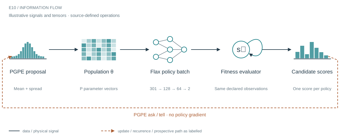
The architecture in context
The system we are building
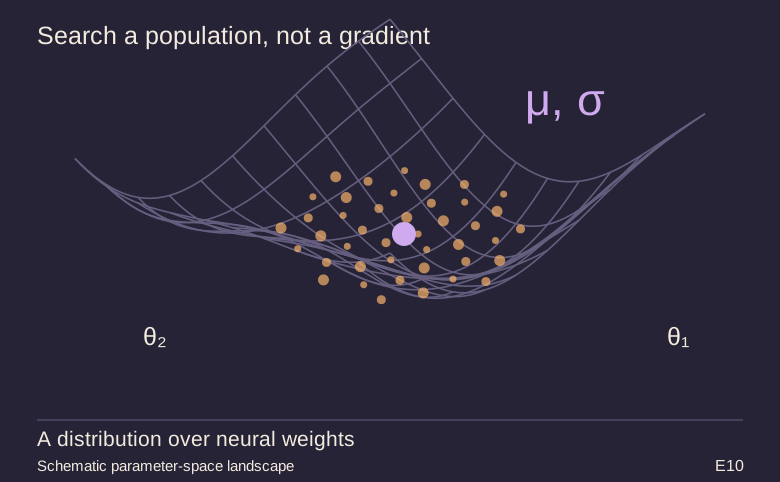
Neuroevolution evaluates many candidate parameter vectors instead of differentiating a reward through a simulator. This notebook explores several implementations; the selected PGPE path combines a Flax policy with a vectorized task evaluator. JAX vmap maps one individual evaluator over the population axis, keeping the meaning of an individual evaluation explicit.
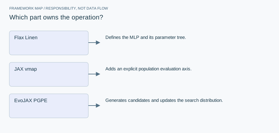
Who does what in the stack
- Flax Linen
- Defines the MLP and its parameter tree.
- JAX vmap
- Adds an explicit population evaluation axis.
- EvoJAX PGPE
- Generates candidates and updates the search distribution.
Custom PolicyNetwork and VectorizedTask adapters translate between flat optimizer vectors, structured Flax parameters, observations and fitness scores. The notebook also contains earlier CMA-ES, MLX and PyTorch experiments. Their presence documents exploration; it is not a controlled cross-backend speed comparison.
From module map to executable structure
Inside Flax policy optimized by PGPE
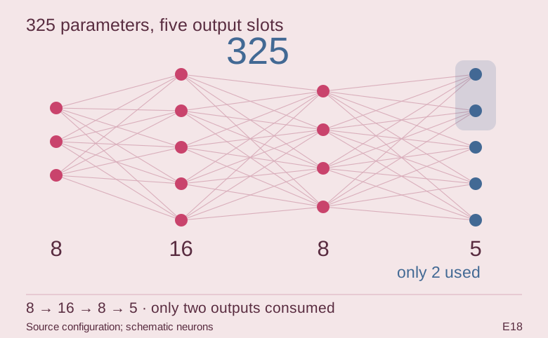
Selected network definition: input dimension configurable (default 301), hidden widths 128 and 64, two outputs.
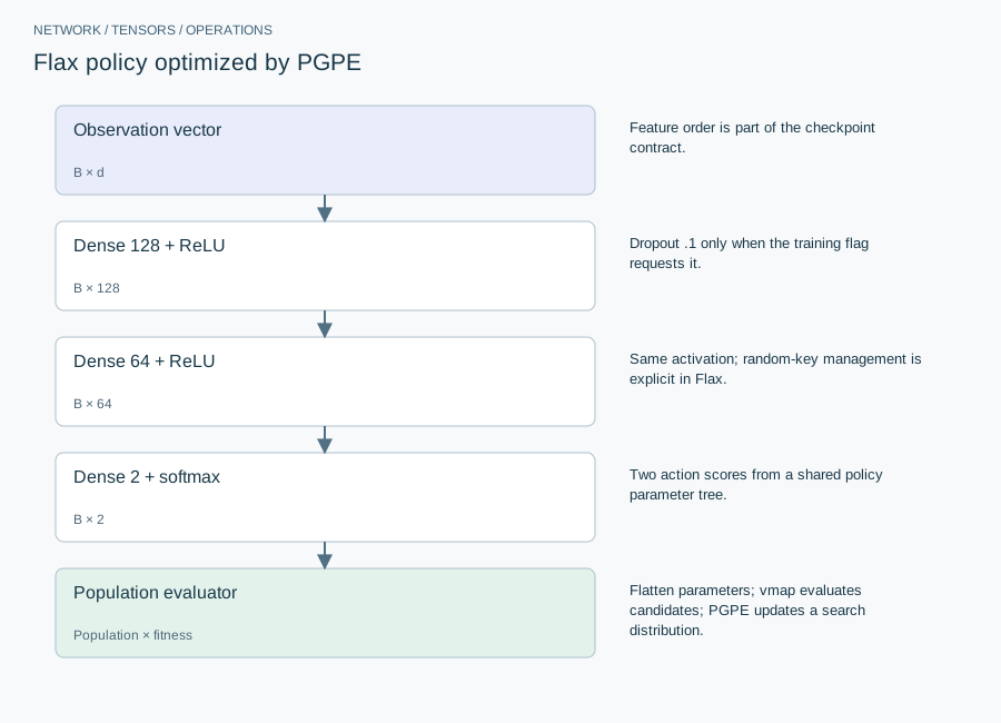
| Layer or branch | Output shape | Implementation detail |
|---|---|---|
| Observation vector | B × d | Feature order is part of the checkpoint contract. |
| Dense 128 + ReLU | B × 128 | Dropout .1 only when the training flag requests it. |
| Dense 64 + ReLU | B × 64 | Same activation; random-key management is explicit in Flax. |
| Dense 2 + softmax | B × 2 | Two action scores from a shared policy parameter tree. |
| Population evaluator | Population × fitness | Flatten parameters; vmap evaluates candidates; PGPE updates a search distribution. |
Flax owns the parameter tree and forward pass. JAX vmap maps the same evaluation function over candidates; it does not make variable-length Python side effects magically vectorized. PGPE changes the distribution over weights using fitness evaluations. A gradient of the network’s logits is not required for that search.
The equation and the update
PGPE uses rollout fitness, not backpropagation through a supervised loss. Population size, rollout count and generation budget determine evaluation work; the selected notebook contains multiple runners, not one uniquely identified benchmark.
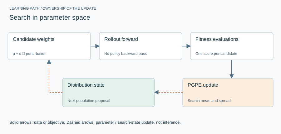
Implementation card / no invented benchmarks
Capacity, budget and execution evidence
- Parameters / retained state
- 47,042 policy scalars when d=301; general count 128(d+1)+64×129+2×65.
- Duration and hardware evidence
- No single source-backed training duration applies to all notebook runners.
- Source coordinates
- E10 cell 9, network definition and population fitness evaluator
- Current reproduction context
- Current workstation, supplied by the author: Apple M4, 128 GB unified RAM, 40 GPU cores and 16 CPU cores. This is context for prospective reproduction, not attribution of every archived run. Python and framework versions are not fully locked for these historical sources; declarations, when available, are identified separately.
Counts above are calculated from the stated layer shapes unless identified as saved measurements. They exclude optimizer state and nontrainable buffers. No archived training was rerun for this revision.
What these design choices change
A small fixed MLP makes the flat search vector manageable. Doubling hidden width can substantially increase both the search dimension and population evaluation memory. Dropout noise and environment noise must be separated from perturbation noise or candidate rankings become needlessly variable.
Reproduction and measurement protocol
Round-trip the parameter pytree through flatten/unflatten and compare outputs exactly before running a population. Evaluate the same candidate and random seed twice. Time compilation separately from warm evaluation, and report candidates times rollout steps rather than calling a generation equivalent to a supervised epoch.
For a new run, save the resolved Python/framework versions, backend, dtype, seed, input shapes, batch size and exact source revision. Start with one batch and one update. Log training steps separately from epochs or environment steps. Do not equate the configured maximum with a completed budget or convergence.
Measure initialization/compilation, data preparation, warmed forward pass, training updates and evaluation separately. Synchronize accelerator work around timed regions using the chosen framework’s supported mechanism. Report peak process memory and framework allocation separately; parameter bytes exclude activations, gradients, optimizer state and input buffers. On a shared machine, begin with a single CPU worker and a small batch rather than claiming all available resources.
A closer look at the implementation
The code that carries the idea
The snippet returns one scalar fitness per parameter vector. The vectorization boundary is the candidate, not a time step or a training batch. Parameters are supplied as data to the policy rather than mutated inside a shared model object. This is the key to avoiding accidental state sharing across candidates.
    def evaluate_population(self,
                           policy: EntryDetectionPolicy,
                           params_batch: jnp.ndarray) -> jnp.ndarray:
        """
        Evaluate population fitness in batch

        Args:
            policy: Policy network
            params_batch: Parameter vectors (pop_size, param_dim)

        Returns:
            fitness_scores: Fitness for each individual (pop_size,)
        """
        pop_size = params_batch.shape[0]

        # Evaluate each individual using vectorized operations
        fitness_scores = jax.vmap(
            lambda params: self._evaluate_individual(policy, params)
        )(params_batch)

        return fitness_scores
Verbatim archive excerpt from evojax_tests.ipynb. Context-dependent historical code, not a standalone runnable program. Comments retain their original wording; the article distinguishes implemented behavior from stale or overbroad comments.
The boundary that matters
The notebook’s own expansion of the PGPE acronym is not authoritative; the article uses the established algorithm name without repeating it. Device detection also does not prove that every operation runs efficiently on that backend. Warm-up, compilation, host copies and candidate memory belong in a performance measurement.