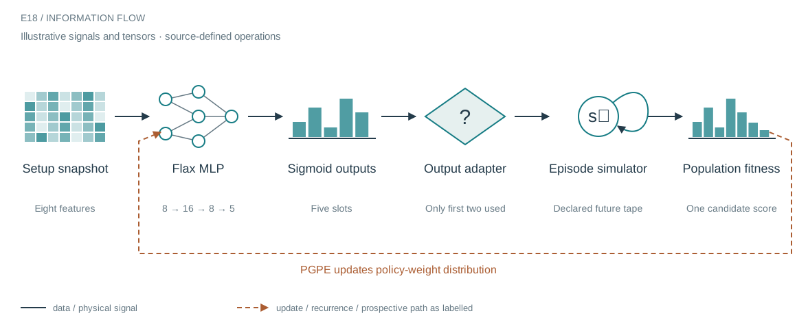
The architecture in context
The system we are building
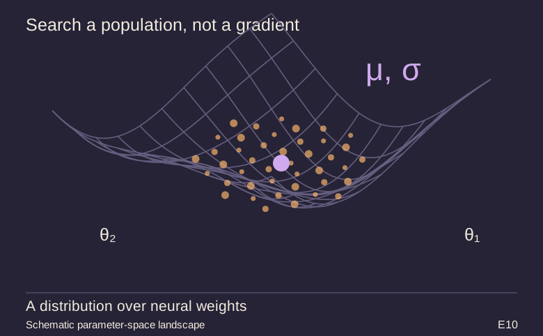
A Flax network has a tree of parameter arrays; an evolutionary optimizer usually proposes flat vectors. The policy adapter initializes a template network, obtains a reversible flattening function and reconstructs a parameter tree for each candidate. This keeps the model definition independent of the search algorithm.
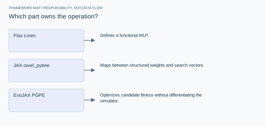
Who does what in the stack
- Flax Linen
- Defines a functional MLP.
- JAX ravel_pytree
- Maps between structured weights and search vectors.
- EvoJAX PGPE
- Optimizes candidate fitness without differentiating the simulator.
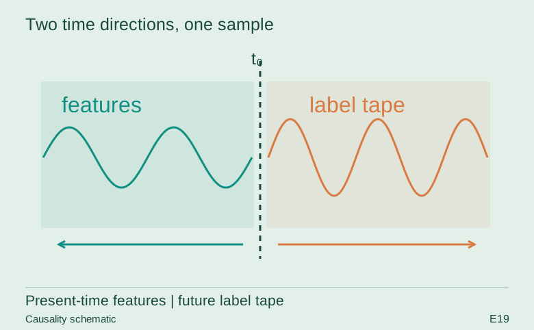
The project combines a Linen MLP, an EvoJAX policy interface and a vectorized episode simulator. The simulator uses scan-like state propagation over a future tape to score a fixed decision rule. This is black-box optimization of parameters, not backpropagation through a differentiable environment.
Open up the implementation
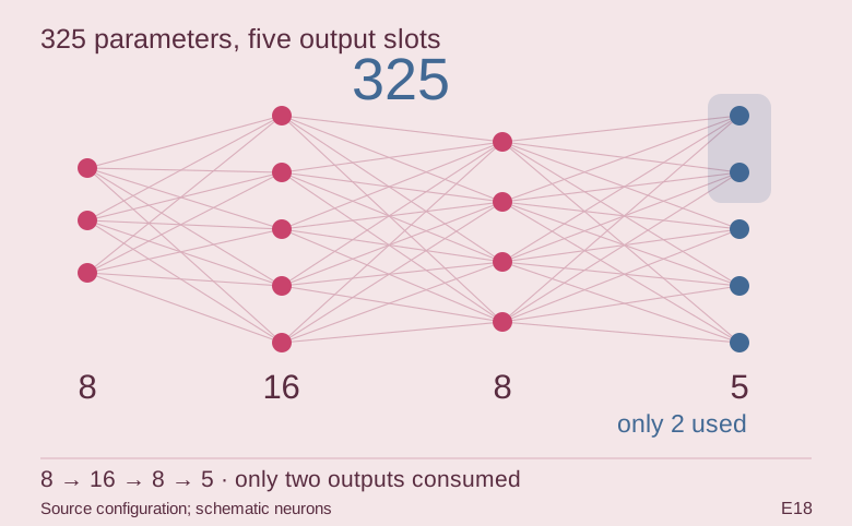
A325-parameter policy with five output slots
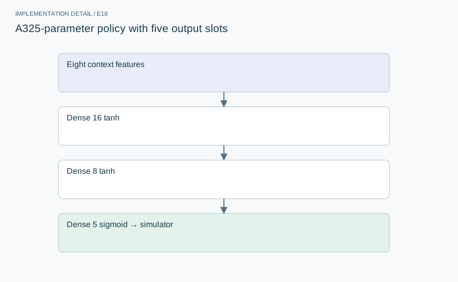
Flax Linen builds the small MLP, while EvoJAX PGPE optimizes a flattened parameter vector. The simulator consumes only two output coordinates in the inspected active path. Five sigmoid outputs therefore do not establish five learned controls; the remaining coordinates and their corresponding weights can be inactive with respect to fitness.
The mathematical contract
Small parameter count can make population search affordable, but total cost is population times generations times simulated opportunities. Reducing unused outputs is a sensible separately tested refactor, not evidence that the archived search found a profitable strategy. Bounded sigmoid values still require a precisely documented mapping to physical simulator units.
Implementation and resource card
- Capacity / budget
- For eight inputs and hidden 16/8:144+136+45=325 parameters. Configured population 256,1,000 generations; PGPE center rate .05, spread rate .1, noise .3, dropout 0.
- Execution evidence
- This revision inspects and explains the archived implementation. It does not rerun the original workload. No unrecorded convergence time, throughput or accelerator result is supplied.
- Current reproduction context
- Current workstation, supplied by the author: Apple M4, 128 GB unified RAM, 40 GPU cores and 16 CPU cores. This is context for prospective reproduction, not attribution of every archived run. Python and framework versions are not fully locked for these historical sources; declarations, when available, are identified separately.
From explanation to a reproducible check
Perturb one output-head row at a time and check whether the simulator result changes. Round-trip the flattened weights and evaluate a fixed input. Count effective parameters separately from allocated parameters and keep all outcome claims within the historical simulation assumptions.
Preserve input identities, configuration and failure records with the result. A successful numerical check only establishes the operation it exercises: it does not certify an entire dataset, model or deployed system. Reproduce the interface on a small deterministic input before optimizing throughput or increasing workload size.
A closer look at the implementation
The code that carries the idea
ravel_pytree returns both the flat coordinates and an unravel function. The latter retains the template’s shapes and tree structure. get_actions reconstructs the candidate parameters and passes them into model.apply, avoiding mutation of a single global model between candidates.
    def _get_param_info(self, params):
        # Call directly from the module
        flat_params, unravel_fn = jax.flatten_util.ravel_pytree(params)
        return len(flat_params), unravel_fn

    def get_actions(self, t_states, params, p_states):
        # params is flat, need to unravel
        model_params = self.format_params_fn(params)
        return self.model.apply(model_params, t_states.obs), p_states
Verbatim archive excerpt from train_umbrella_pgpe.py. Context-dependent historical code, not a standalone runnable program. Comments retain their original wording; the article distinguishes implemented behavior from stale or overbroad comments.
The boundary that matters
The archived network produces five sigmoid outputs, but the inspected active simulation consumes only its first two. Unused outputs add search dimensions without affecting fitness. Simulator boundary ordering is declared code behavior, not evidence of tick-level execution or achievable P&L.