The architecture in context
The system we are building
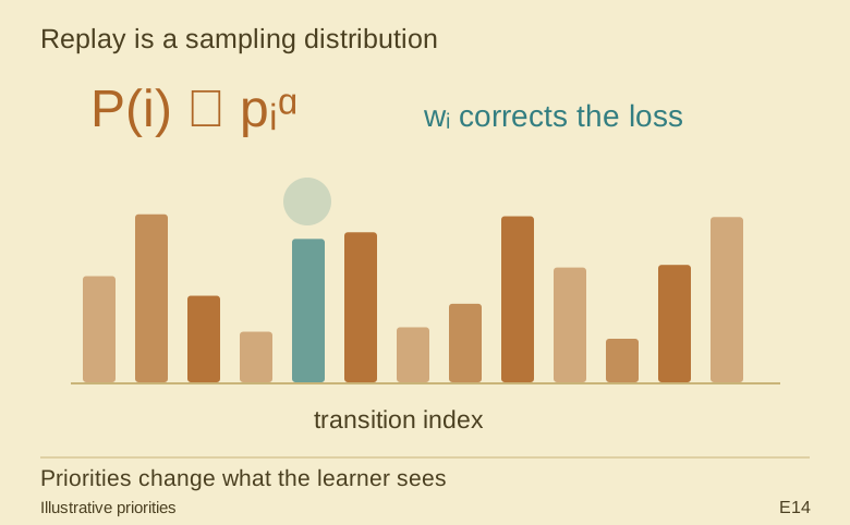
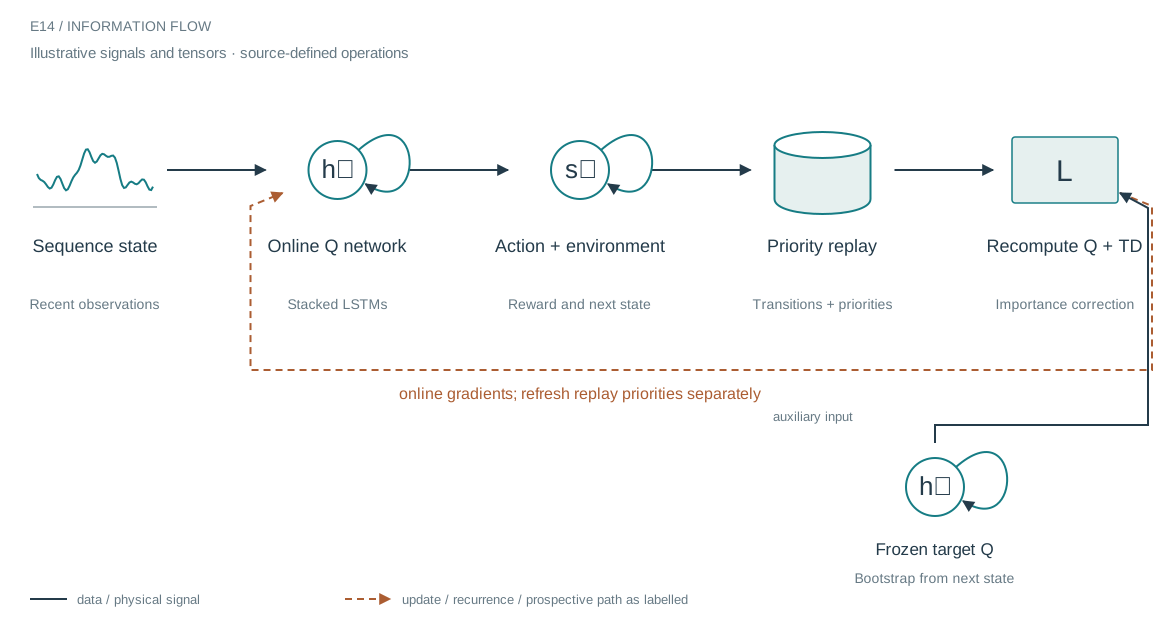
Replay decouples data collection from gradient updates. Prioritized replay goes further: transitions with larger recorded priorities are sampled more often. The high-frequency DQN notebook wraps this mechanism around a recurrent Q network, with an explicit target network and soft updates. A sampled item still has to represent a coherent transition; priority must not change temporal alignment.
Who does what in the stack
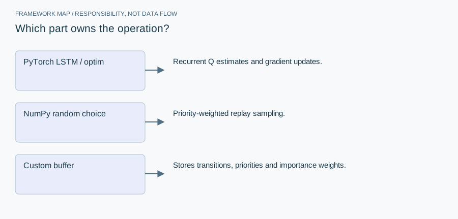
- PyTorch LSTM / optim
- Recurrent Q estimates and gradient updates.
- NumPy random choice
- Priority-weighted replay sampling.
- Custom buffer
- Stores transitions, priorities and importance weights.
A custom replay buffer owns priorities, sampling indices, importance weights and the beta schedule. PyTorch owns the LSTM and optimizer. NumPy samples the replay indices. This separation makes it possible to test the buffer independently from an expensive environment run.
From module map to executable structure
Inside Recurrent Q-network
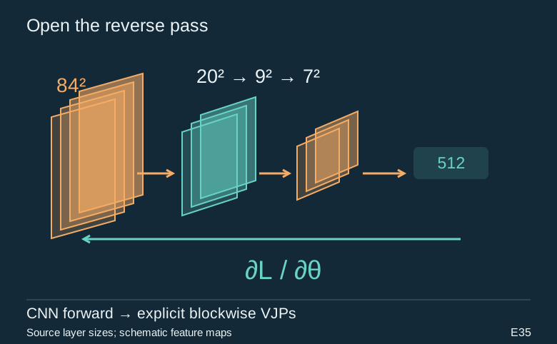
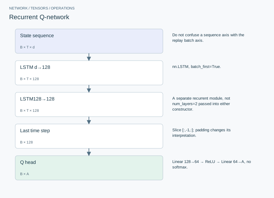
Two single-layer PyTorch LSTMs, hidden 128; configurable observation and action dimensions.
| Layer or branch | Output shape | Implementation detail |
|---|---|---|
| State sequence | B × T × d | Do not confuse a sequence axis with the replay batch axis. |
| LSTM d→128 | B × T × 128 | nn.LSTM, batch_first=True. |
| LSTM128→128 | B × T × 128 | A separate recurrent module, not num_layers=2 passed into either constructor. |
| Last time step | B × 128 | Slice [:,-1,:]; padding changes its interpretation. |
| Q head | B × A | Linear 128→64 → ReLU → Linear 64→A, no softmax. |
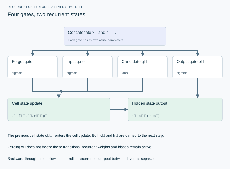
The recurrent encoder converts a window into one feature vector; the head estimates one action value per action, not action probabilities. The target network supplies a slowly changing bootstrap. Stop-gradient applies to the target, while only the taken action contributes to each sampled TD error.
The equation and the update
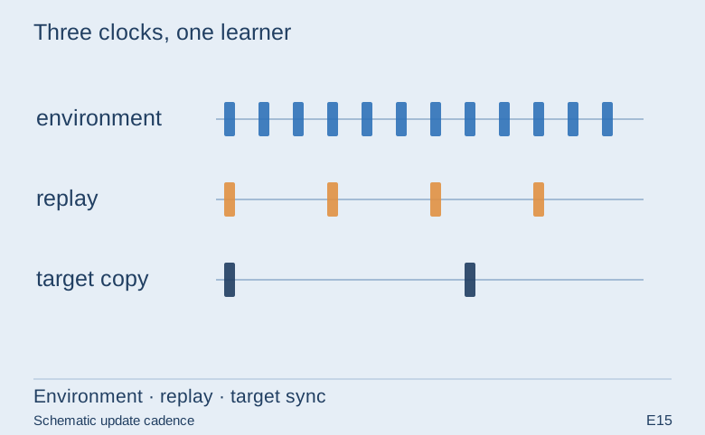
Defaults: Adam 1e-3, gamma .99, replay 50,000 and batch 128. E14 adds prioritized replay and soft target updates (tau .005); E15 uses its own replay/target-update logic. They are not interchangeable training protocols.
Implementation card / no invented benchmarks
Capacity, budget and execution evidence
- Parameters / retained state
- 512(d+130)+512×258+8,256+65A per network, using PyTorch’s two bias vectors. Target network duplicates stored parameters.
- Duration and hardware evidence
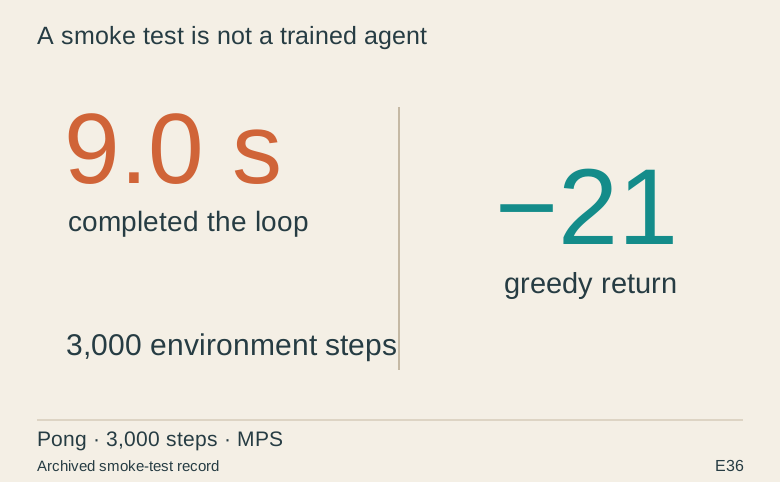
- Archived examples are limited/interrupted runs; no convergence speed is inferred.
- Source coordinates
- E14 cell 2, lines 315–363; E15 cell 5, lines 39–80
- Current reproduction context
- Current workstation, supplied by the author: Apple M4, 128 GB unified RAM, 40 GPU cores and 16 CPU cores. This is context for prospective reproduction, not attribution of every archived run. Python and framework versions are not fully locked for these historical sources; declarations, when available, are identified separately.
Counts above are calculated from the stated layer shapes unless identified as saved measurements. They exclude optimizer state and nontrainable buffers. No archived training was rerun for this revision.
What these design choices change
Longer windows enlarge unrolled activation memory without changing the count of recurrent weights. Prioritized replay changes the sample distribution, so importance weights belong inside the per-sample loss before reduction. A priority exponent and an importance exponent serve different purposes.
Reproduction and measurement protocol
Create one terminal and one nonterminal transition and calculate both targets by hand. Test that priority updates use the intended TD-error magnitude. For recurrent replay, declare whether hidden state is reset for each sampled window; state carried across unrelated samples is a different algorithm.
For a new run, save the resolved Python/framework versions, backend, dtype, seed, input shapes, batch size and exact source revision. Start with one batch and one update. Log training steps separately from epochs or environment steps. Do not equate the configured maximum with a completed budget or convergence.
Measure initialization/compilation, data preparation, warmed forward pass, training updates and evaluation separately. Synchronize accelerator work around timed regions using the chosen framework’s supported mechanism. Report peak process memory and framework allocation separately; parameter bytes exclude activations, gradients, optimizer state and input buffers. On a shared machine, begin with a single CPU worker and a small batch rather than claiming all available resources.
A closer look at the implementation
The code that carries the idea
The snippet raises priorities to alpha, normalizes them into a distribution and samples with replacement. The weight (N p_i)^(-beta) downweights heavily sampled transitions; normalization by the largest sampled weight controls scale. The sampled indices must return to the buffer when new TD errors update priorities.
    def sample(self, batch_size):
        if len(self.memory) < batch_size:
            return None

        # Calculate sampling probabilities
        probs = self.priorities[:len(self.memory)] ** self.alpha
        probs /= probs.sum()

        # Sample indices based on priorities
        indices = np.random.choice(len(self.memory), batch_size, p=probs)

        # Calculate importance sampling weights
        weights = (len(self.memory) * probs[indices]) ** (-self.beta)
        weights /= weights.max()
        weights = torch.FloatTensor(weights)

        # Increase beta
        self.beta = min(1.0, self.beta + self.beta_increment)

        batch = [self.memory[idx] for idx in indices]
        batch = Transition(*zip(*batch))

        return batch, indices, weights
Verbatim archive excerpt from pt_drl_high_freq.ipynb. Context-dependent historical code, not a standalone runnable program. Comments retain their original wording; the article distinguishes implemented behavior from stale or overbroad comments.
The boundary that matters
Repeated indices in a batch are valid under this sampler. Zero or nonfinite total priority is not. The archive contains a partial interrupted run, so this article explains an implementation rather than claiming learning success or improved returns.