The architecture in context
What this comparison asks
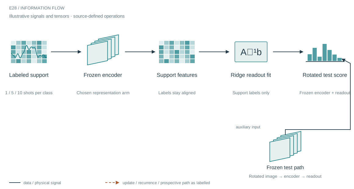
An invariant representation should reduce how many labeled examples are needed across transformations. The saved experiment places labeled support examples near a canonical orientation and evaluates on broadly rotated images. This is a harder and more specific question than ordinary IID digit classification.
Who does what in the stack
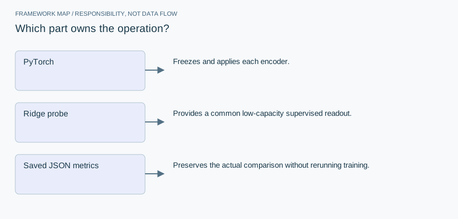
- PyTorch
- Freezes and applies each encoder.
- Ridge probe
- Provides a common low-capacity supervised readout.
- Saved JSON metrics
- Preserves the actual comparison without rerunning training.
The companion evaluator controls support counts, rotation policy and frozen-feature fitting. The primary evidence for this article is the saved metrics file; the code excerpt comes from the implementation that constructs the evaluation. Those are complementary artifacts, not two independent experiments.
From module map to executable structure
Inside Contrastive image encoder
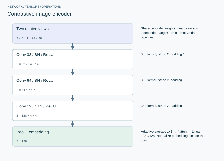
This results or evaluation article shares the implementation in E27. The architecture below describes that companion, not a newly trained model.
Rotating MNIST; grayscale input 28×28; embedding 128.
| Layer or branch | Output shape | Implementation detail |
|---|---|---|
| Two rotated views | 2 × B × 1 × 28 × 28 | Shared encoder weights; nearby versus independent angles are alternative data pipelines. |
| Conv 32 / BN / ReLU | B × 32 × 14 × 14 | 3×3 kernel, stride 2, padding 1. |
| Conv 64 / BN / ReLU | B × 64 × 7 × 7 | 3×3 kernel, stride 2, padding 1. |
| Conv 128 / BN / ReLU | B × 128 × 4 × 4 | 3×3 kernel, stride 2, padding 1. |
| Pool + embedding | B × 128 | Adaptive average 1×1 → flatten → Linear 128→128. Normalize embeddings inside the loss. |
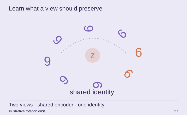
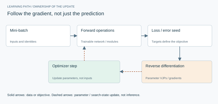
The diagonal of the B×B cross-view similarity matrix contains positive pairs. Other columns are negatives for that row. Both directions contribute. Labels are not used for encoder training but are used in the downstream ridge probe. The two views must be different transforms of the same original digit, not independently sampled digit identities.
The equation and the update
Adam 1e-3; batch 256; temperature .2. Script default 20 epochs / temporal angle window 20°. E28’s saved comparison instead records 25 epochs / window 60° and a canonical probe. The distinction must survive reproduction.
Implementation card / no invented benchmarks
Capacity, budget and execution evidence
- Parameters / retained state
- 109,632 trainable scalars; BatchNorm running statistics are separate buffers.
- Duration and hardware evidence
- The saved JSON does not contain a verified end-to-end timing.
- Source coordinates
- E27 lines 23–25, 45–71 and 115–148
- Current reproduction context
- Current workstation, supplied by the author: Apple M4, 128 GB unified RAM, 40 GPU cores and 16 CPU cores. This is context for prospective reproduction, not attribution of every archived run. Python and framework versions are not fully locked for these historical sources; declarations, when available, are identified separately.
Counts above are calculated from the stated layer shapes unless identified as saved measurements. They exclude optimizer state and nontrainable buffers. No archived training was rerun for this revision.
What these design choices change
The channel expansion compensates for shrinking spatial resolution; global pooling discards spatial location before the probe. Temperature controls the sharpness of relative similarities. Increasing batch size changes both optimization and the number of negatives, so it is not purely a throughput change.
Reproduction and measurement protocol
Check pair indices before augmenting, compute the similarity matrix on a tiny batch, and verify that swapping both view orders together leaves the symmetric loss unchanged. Freeze the encoder and set eval mode before few-shot embedding extraction; otherwise BatchNorm updates contaminate the probe protocol.
For a new run, save the resolved Python/framework versions, backend, dtype, seed, input shapes, batch size and exact source revision. Start with one batch and one update. Log training steps separately from epochs or environment steps. Do not equate the configured maximum with a completed budget or convergence.
Measure initialization/compilation, data preparation, warmed forward pass, training updates and evaluation separately. Synchronize accelerator work around timed regions using the chosen framework’s supported mechanism. Report peak process memory and framework allocation separately; parameter bytes exclude activations, gradients, optimizer state and input buffers. On a shared machine, begin with a single CPU worker and a small batch rather than claiming all available resources.
A closer look at the implementation
The code that carries the idea
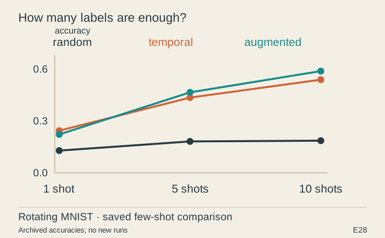
The excerpt separates support sampling, feature extraction and ridge probing. This lets the representation be assessed with the same low-capacity readout. The saved canonical ten-shot accuracies are 0.186 for the random encoder, 0.539 for temporal pairing and 0.5887 for independent augmentation.
def few_shot_eval(enc, Xtr, ytr, Xte, yte, K, canon=False, seed=0):
    """K labeled examples/class (support at canonical angle if canon, else random); test on ALL-angle test set."""
    g = torch.Generator(device="cpu"); g.manual_seed(seed); idx = []
    yc = ytr.cpu()
    for c in range(NC):
        ci = (yc == c).nonzero().flatten(); idx.append(ci[torch.randperm(len(ci), generator=g)[:K]])
    idx = torch.cat(idx).to(DEV)
    Xs = rotate(Xtr[idx], support_angles(len(idx), canon)); ys = ytr[idx]
    aT = torch.rand(len(Xte), device=DEV) * 360.0; Xt = rotate(Xte, aT)                  # test ALWAYS spans all angles
    Fs = embed(enc, Xs); Ft = embed(enc, Xt)
    return ridge_probe(Fs, ys, Ft, yte)
Verbatim archive excerpt from closed_form_neat_invariance.py (companion source E27). Context-dependent historical code, not a standalone runnable program. Comments retain their original wording; the article distinguishes implemented behavior from stale or overbroad comments.
The saved comparison
Archived results, not new training. The article states the comparison’s scope and limitations.
| Encoder | 1 shot | 5 shots | 10 shots |
|---|---|---|---|
| Random | 0.1287 | 0.1817 | 0.1860 |
| Temporal | 0.2440 | 0.4353 | 0.5390 |
| Augmented | 0.2220 | 0.4657 | 0.5887 |
The boundary that matters
The temporal representation improves over random features in this saved comparison, but does not beat the augmentation control at ten shots. The figures are archived point results, not newly reproduced confidence intervals or proof of universal data efficiency.