The architecture in context
What this comparison asks
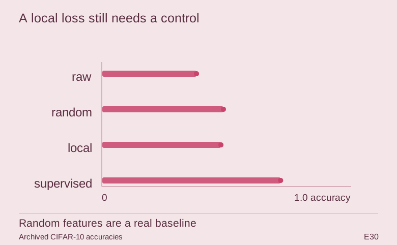
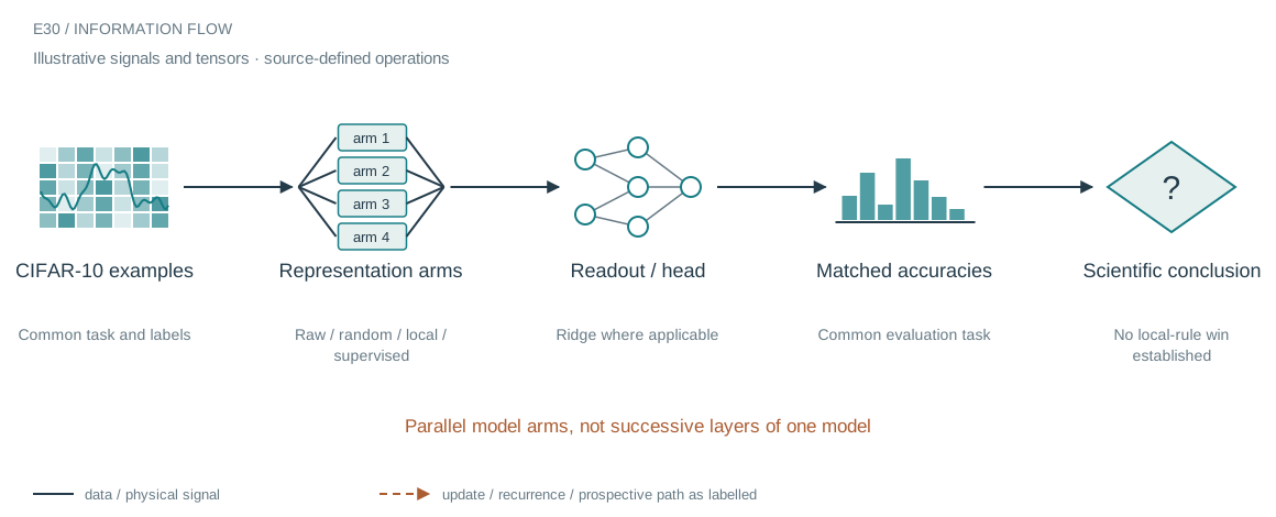
The blockwise contrastive experiment produced a representation, but the relevant question is whether it improved the downstream task. The saved comparison includes raw features, a random convolutional representation and supervised training. That makes it possible to distinguish the value of the architecture from the value of the local learning rule.
Who does what in the stack
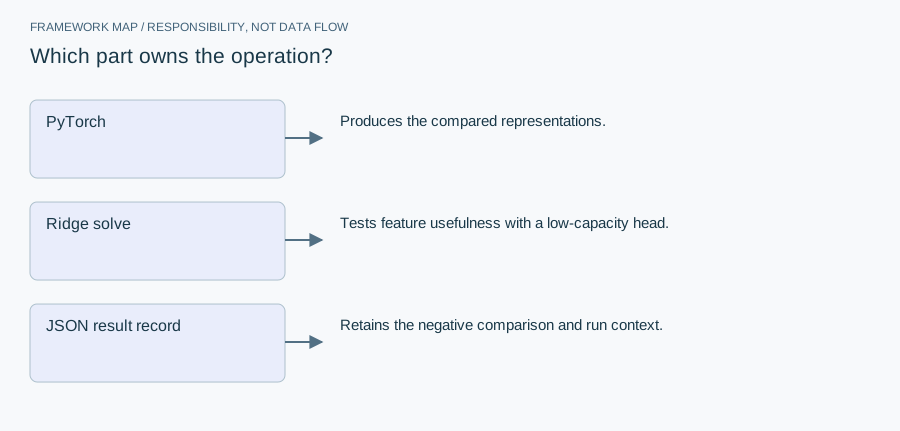
- PyTorch
- Produces the compared representations.
- Ridge solve
- Tests feature usefulness with a low-capacity head.
- JSON result record
- Retains the negative comparison and run context.
The evaluation code fits a ridge readout after training the representation, using training-derived feature normalization. The result file records the arm outputs and run context. This article is a case study in interpreting a failed learning recipe, not a second implementation of the blockwise network.
From module map to executable structure
Inside Greedy local contrastive CNN
This results or evaluation article shares the implementation in E29. The architecture below describes that companion, not a newly trained model.
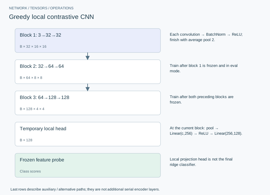
CIFAR-10, three blocks with channels 32,64,128; two 3×3 convolutions per block.
| Layer or branch | Output shape | Implementation detail |
|---|---|---|
| Block 1: 3→32→32 | B × 32 × 16 × 16 | Each convolution → BatchNorm → ReLU; finish with average pool 2. |
| Block 2: 32→64→64 | B × 64 × 8 × 8 | Train after block 1 is frozen and in eval mode. |
| Block 3: 64→128→128 | B × 128 × 4 × 4 | Train after both preceding blocks are frozen. |
| Temporary local head | B × 128 | At the current block: pool → Linear(c,256) → ReLU → Linear(256,128). |
| Frozen feature probe | Class scores | Local projection head is not the final ridge classifier. |
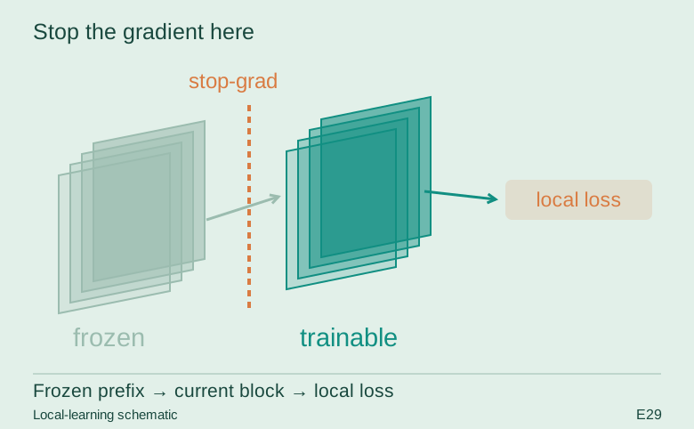
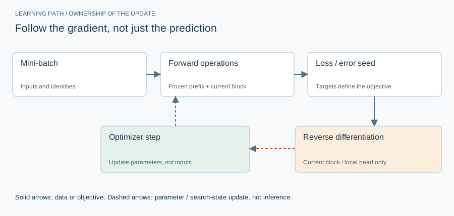
This is a different learning rule from a blockwise reverse sweep. A local loss updates only the current block and its projection head. Previously trained blocks receive neither an input gradient nor an optimizer step. The NT-Xent matrix contains 2B views, excludes self-similarity and identifies the matching view by a half-batch offset.
The equation and the update
Configured 80 epochs per block, batch 512, Adam 1e-3, temperature .2; subset 20,000. The saved comparison is negative versus random convolutional features. Do not reinterpret the training budget as evidence of a benefit.
Implementation card / no invented benchmarks
Capacity, budget and execution evidence
- Parameters / retained state
- 287,904 backbone scalars. Each temporary projection head adds 256(c+1)+128×257; heads are not all simultaneously trained.
- Duration and hardware evidence
- E30 records 326.8 seconds for its saved experiment on MPS; this is not a per-block or per-epoch timing and does not identify the current workstation.
- Source coordinates
- E29 lines 24–25 and 50–84
- Current reproduction context
- Current workstation, supplied by the author: Apple M4, 128 GB unified RAM, 40 GPU cores and 16 CPU cores. This is context for prospective reproduction, not attribution of every archived run. Python and framework versions are not fully locked for these historical sources; declarations, when available, are identified separately.
Counts above are calculated from the stated layer shapes unless identified as saved measurements. They exclude optimizer state and nontrainable buffers. No archived training was rerun for this revision.
What these design choices change
Greedy freezing can reduce simultaneously trainable state but may discard information that later blocks need. A useful local contrastive objective is not automatically a useful end-to-end representation. The supervised and random-feature controls are necessary to interpret the negative result.
Reproduction and measurement protocol
After one optimizer step, compare every earlier block’s parameters and BatchNorm buffers byte-for-byte. Check that only the current block and projection head move. A zero parameter gradient is insufficient if running statistics continue changing.
For a new run, save the resolved Python/framework versions, backend, dtype, seed, input shapes, batch size and exact source revision. Start with one batch and one update. Log training steps separately from epochs or environment steps. Do not equate the configured maximum with a completed budget or convergence.
Measure initialization/compilation, data preparation, warmed forward pass, training updates and evaluation separately. Synchronize accelerator work around timed regions using the chosen framework’s supported mechanism. Report peak process memory and framework allocation separately; parameter bytes exclude activations, gradients, optimizer state and input buffers. On a shared machine, begin with a single CPU worker and a small batch rather than claiming all available resources.
A closer look at the implementation
The code that carries the idea
The companion snippet fits the classifier in feature space. The archived local-learning accuracy is 0.4907, slightly below random convolutional features at 0.5010 and well below the supervised arm at 0.7376. Raw features reach 0.3896. These values describe the saved setting, not a full sweep of the method family.
def probe(Ftr, ytr, Fte, yte, lam=1e2):
    mu, sd = Ftr.mean(0), Ftr.std(0) + 1e-6; Ftr = (Ftr - mu) / sd; Fte = (Fte - mu) / sd
    Ftr = torch.cat([Ftr, torch.ones(len(Ftr), 1, device=DEV)], 1); Fte = torch.cat([Fte, torch.ones(len(Fte), 1, device=DEV)], 1)
    yoh = torch.eye(10, device=DEV)[ytr]
    W = torch.linalg.solve(Ftr.T @ Ftr + lam * torch.eye(Ftr.shape[1], device=DEV), Ftr.T @ yoh)
    return float((Fte @ W).argmax(1).eq(yte).float().mean())
Verbatim archive excerpt from closed_form_neat_biolocal.py (companion source E29). Context-dependent historical code, not a standalone runnable program. Comments retain their original wording; the article distinguishes implemented behavior from stale or overbroad comments.
The saved comparison
Archived results, not new training. The article states the comparison’s scope and limitations.
| Arm | Saved accuracy |
|---|---|
| Raw features | 0.3896 |
| Random CNN | 0.5010 |
| Local contrastive | 0.4907 |
| Supervised | 0.7376 |
The boundary that matters
The result does not establish that local learning is impossible, but it does remove the basis for claiming that this particular recipe improved representation quality. More epochs or another projection head would be a new experiment, not a correction to the saved evidence.