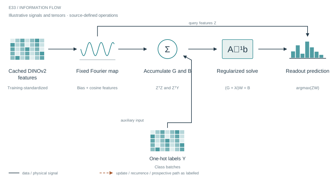
The architecture in context
The system we are building
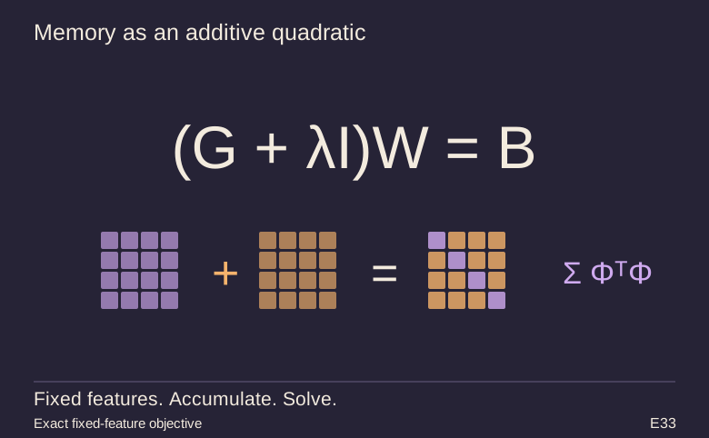
Once the feature map is fixed, ridge regression can be reconstructed from additive statistics rather than all individual examples. The experiment expands cached visual features with a random Fourier map, accumulates a Gram matrix and label cross-products across class batches, then solves a regularized linear system. The accumulation is equivalent to the pooled fixed-feature objective in exact arithmetic.
Who does what in the stack
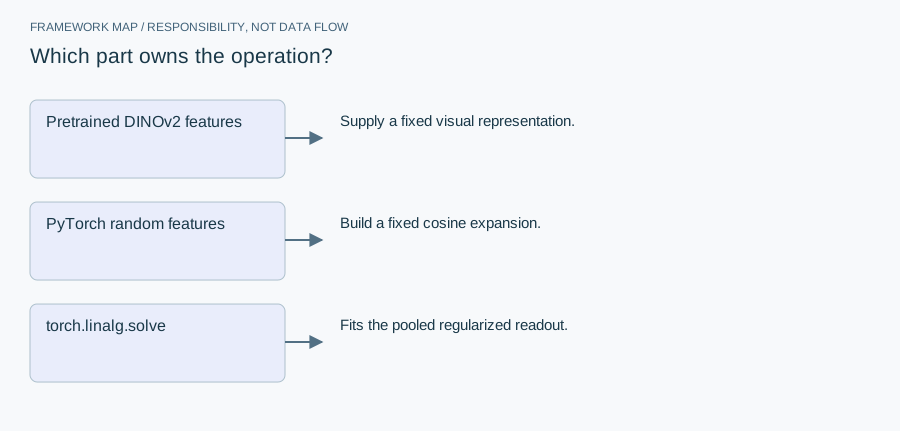
- Pretrained DINOv2 features
- Supply a fixed visual representation.
- PyTorch random features
- Build a fixed cosine expansion.
- torch.linalg.solve
- Fits the pooled regularized readout.
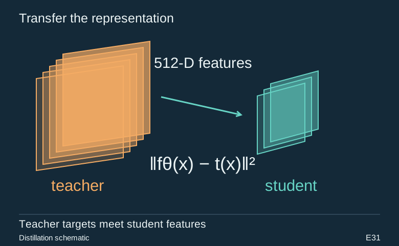
The project combines a pretrained visual encoder with a task-wise readout update and explicit joint-fit controls. It is not teacher-weight distillation: the encoder remains a required feature generator for new images. The custom work is the representation adapter and the experiment around additive learning.
From module map to executable structure
Inside Frozen encoder with additive Gram readout
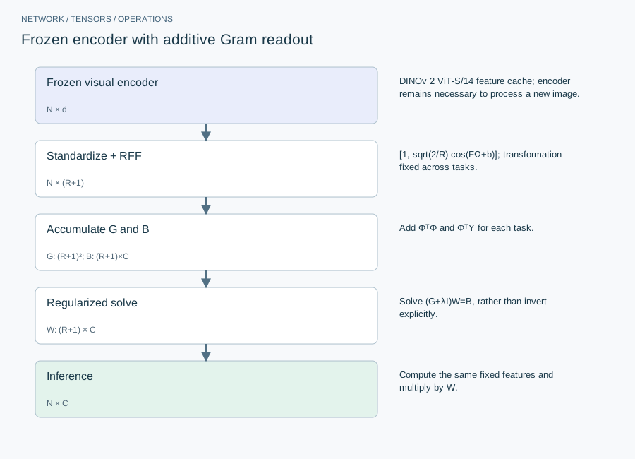
Cached DINOv 2 features → R random Fourier features plus bias; default R=10,000, ten class-incremental tasks.
| Layer or branch | Output shape | Implementation detail |
|---|---|---|
| Frozen visual encoder | N × d | DINOv 2 ViT-S/14 feature cache; encoder remains necessary to process a new image. |
| Standardize + RFF | N × (R+1) | [1, sqrt(2/R) cos(FΩ+b)]; transformation fixed across tasks. |
| Accumulate G and B | G: (R+1)²; B: (R+1)×C | Add ΦᵀΦ and ΦᵀY for each task. |
| Regularized solve | W: (R+1) × C | Solve (G+λI)W=B, rather than invert explicitly. |
| Inference | N × C | Compute the same fixed features and multiply by W. |
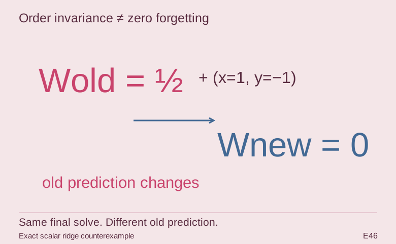
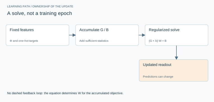
The additive objects are sufficient statistics for one fixed quadratic objective. Associativity removes task-order dependence of that objective, up to floating-point effects. It does not freeze predictions after adding a new task: W is solved again and can change everywhere. A growing or retrained encoder invalidates the old statistics unless their cross-products are reconstructed.
The equation and the update
No SGD epochs for the readout solve. Default ridge λ=10; additive statistics are order-invariant in exact arithmetic for a fixed feature map. Feature standardization uses the full training pool, so this is not a strictly online unknown-future preprocessing protocol.
Implementation card / no invented benchmarks
Capacity, budget and execution evidence
- Parameters / retained state
- Readout has(R+1)C coefficients; G has(R+1)² entries. For R=10,000, float 32 G alone is 400,080,004 bytes. Frozen encoder weights are additional.
- Duration and hardware evidence
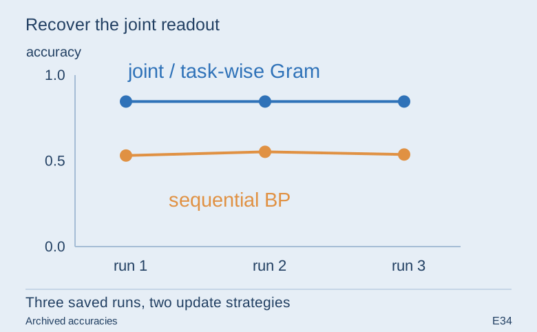
- Saved accuracies support the particular comparison, not a measured edge-device latency or memory-free training claim.
- Source coordinates
- E33 feature transformation, accumulator and ridge solve; E34 saved metrics
- Current reproduction context
- Current workstation, supplied by the author: Apple M4, 128 GB unified RAM, 40 GPU cores and 16 CPU cores. This is context for prospective reproduction, not attribution of every archived run. Python and framework versions are not fully locked for these historical sources; declarations, when available, are identified separately.
Counts above are calculated from the stated layer shapes unless identified as saved measurements. They exclude optimizer state and nontrainable buffers. No archived training was rerun for this revision.
What these design choices change
R controls approximation capacity but also quadratic Gram storage and solve cost. Increasing R from 4,000 to 10,000 multiplies G storage by roughly 6.25, even though feature width increases only 2.5 times. A small trainable readout is therefore not the same as a small total-memory training system.
Reproduction and measurement protocol
Compare accumulated G/B with a single concatenated-batch computation in float 64 on a tiny example. Then reverse task order and report coefficient and prediction tolerances. Keep encoder, normalization, RFF seed and ridge convention in the checkpoint; weights alone are not a complete inference artifact.
For a new run, save the resolved Python/framework versions, backend, dtype, seed, input shapes, batch size and exact source revision. Start with one batch and one update. Log training steps separately from epochs or environment steps. Do not equate the configured maximum with a completed budget or convergence.
Measure initialization/compilation, data preparation, warmed forward pass, training updates and evaluation separately. Synchronize accelerator work around timed regions using the chosen framework’s supported mechanism. Report peak process memory and framework allocation separately; parameter bytes exclude activations, gradients, optimizer state and input buffers. On a shared machine, begin with a single CPU worker and a small batch rather than claiming all available resources.
A closer look at the implementation
The code that carries the idea
The excerpt updates G and B inside the task loop and solves only after accumulation. That preserves the information needed for the declared ridge objective, but not arbitrary future features or old-task predictions. With 10,000 Fourier coordinates plus a bias, a dense float32 Gram alone is about 400 MB.
def gram_cil_acc(Ztr, yo, Zte, yeo, tasks, nclass, lam):
    Fdim = Ztr.shape[1]; G = torch.zeros(Fdim, Fdim); B = torch.zeros(Fdim, nclass)
    for cls in tasks:
        m = torch.isin(yo, torch.tensor(cls)); Y = torch.zeros(int(m.sum()), nclass); Y[torch.arange(int(m.sum())), yo[m]] = 1
        G = G + Ztr[m].T @ Ztr[m]; B = B + Ztr[m].T @ Y
    W = torch.linalg.solve(G + lam * torch.eye(Fdim), B)
    return float(((Zte @ W).argmax(1) == yeo).float().mean())
Verbatim archive excerpt from closed_form_distill_frontier.py. Context-dependent historical code, not a standalone runnable program. Comments retain their original wording; the article distinguishes implemented behavior from stale or overbroad comments.
The boundary that matters
Training-wide feature standardization is computed before the simulated task stream. This is a declared full-training preprocessing choice, not a strictly online normalization scheme. Floating-point sums are also not bitwise order-independent.