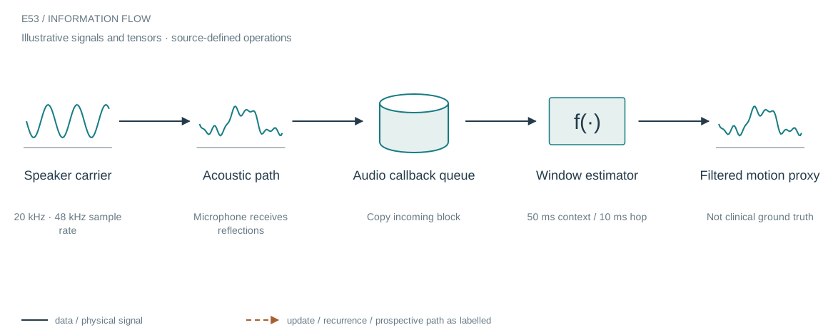
The architecture in context
The system we are building
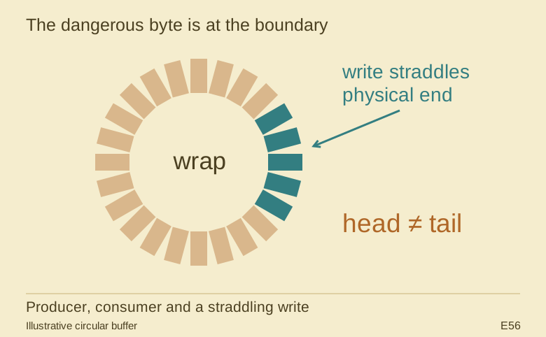
The prototype emits a carrier and processes microphone input to estimate frequency changes. A sounddevice callback supplies output samples and copies input blocks into a queue; the main loop performs estimation and tracking. Separating these paths keeps plotting and heavier processing out of the immediate audio callback.
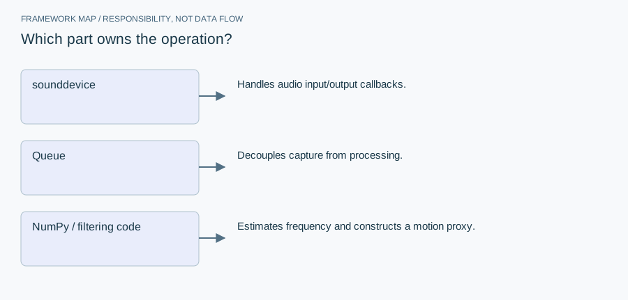
Who does what in the stack
- sounddevice
- Handles audio input/output callbacks.
- Queue
- Decouples capture from processing.
- NumPy / filtering code
- Estimates frequency and constructs a motion proxy.
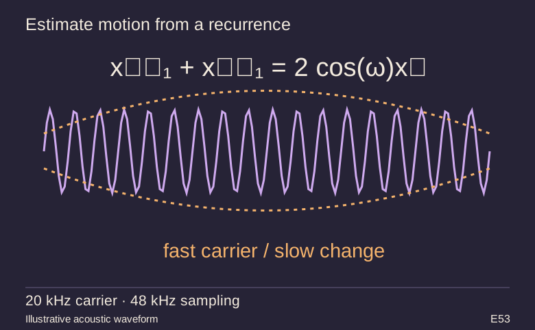
The custom estimator uses the sinusoid recurrence x[n−1]+x[n+1]=2 cos(ωT)x[n]. It aggregates products across a window to estimate cos(ωT), clips the estimate to the arccos domain and converts the angle to a frequency. NumPy supplies the arithmetic; the physical interpretation depends on the measurement setup.
Open up the implementation
A frequency estimator inside an audio callback system
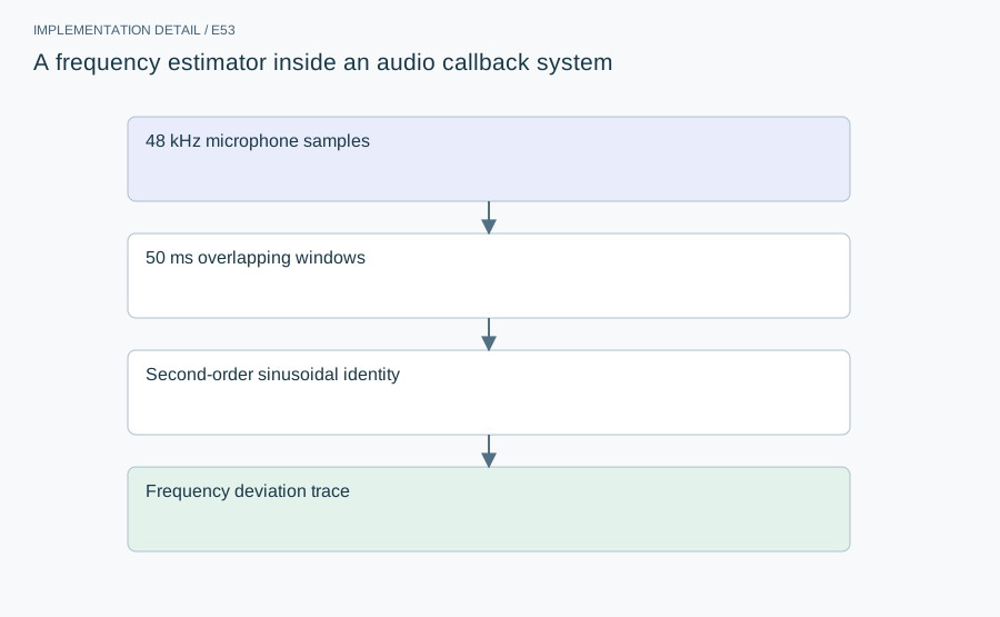
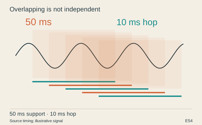
A sinusoid satisfies a second-order recurrence. The estimator fits its cosine coefficient using local products, then converts it to frequency. At 48 kHz, a 50 ms window contains 2,400 samples; a 10 ms hop supplies a 100 Hz update schedule with overlapping information. That is not 100 independent measurements per second.
The mathematical contract
The ratio needs nonzero signal energy and a valid arccos domain. Clipping prevents numerical NaNs but can hide model mismatch. Multiple reflectors, multiple tones and weak signals need quality diagnostics. The active modality is acoustic emission and reception, not Wi-Fi, and a frequency trace is not yet a validated breathing-rate measurement.
Implementation and resource card
- Capacity / budget
- Carrier 20 kHz, sample rate 48 kHz, window 50 ms, hop 10 ms. No neural weights or training epochs; this is a model-based signal estimator.
- Execution evidence
- This revision inspects and explains the archived implementation. It does not rerun the original workload. No unrecorded convergence time, throughput or accelerator result is supplied.
- Current reproduction context
- Current workstation, supplied by the author: Apple M4, 128 GB unified RAM, 40 GPU cores and 16 CPU cores. This is context for prospective reproduction, not attribution of every archived run. Python and framework versions are not fully locked for these historical sources; declarations, when available, are identified separately.
From explanation to a reproducible check
Check a noiseless 20 kHz sinusoid, then add a nearby tone and lower the signal amplitude. Report estimation error and invalid-window rate. A zero-energy fallback to the carrier is an implementation choice, not evidence of a stable physiological signal.
Preserve input identities, configuration and failure records with the result. A successful numerical check only establishes the operation it exercises: it does not certify an entire dataset, model or deployed system. Reproduce the interface on a small deterministic input before optimizing throughput or increasing workload size.
A closer look at the implementation
The code that carries the idea
The denominator is twice the window’s interior signal energy. A zero denominator returns the nominal carrier rather than a reliable new observation. Clipping prevents NaNs, but can hide a poor model fit if it is not accompanied by a quality indicator.
    x_n = x[1:-1]
    x_prev = x[:-2]
    x_next = x[2:]

    num = np.sum((x_prev + x_next) * x_n)
    den = 2.0 * np.sum(x_n**2)

    if den == 0:
        return F_CARRIER

    cos_wT = num / den
    cos_wT = np.clip(cos_wT, -1.0, 1.0)

    wT = np.arccos(cos_wT)
    f_inst = wT / (2 * np.pi * T)
    return f_inst
Verbatim archive excerpt from ghost_v2.py. Context-dependent historical code, not a standalone runnable program. Comments retain their original wording; the article distinguishes implemented behavior from stale or overbroad comments.
The boundary that matters
This is an acoustic experiment, not Wi-Fi sensing. Multiple reflections, carrier leakage, noise and phase discontinuities can violate the single-tone model. A 10 ms hop does not mean a 10 ms independent measurement or validated physiological latency.