Keep tomorrow’s choice open
A small device may finish collecting a long signal before we know the right smoothing time constant. Retaining only the fitted answer closes that choice. Retaining every sample can be expensive. Could the device keep the entire relevant loss landscape instead—a small object that lets us ask a different parameter question after the samples are gone?
What the device keeps after capture
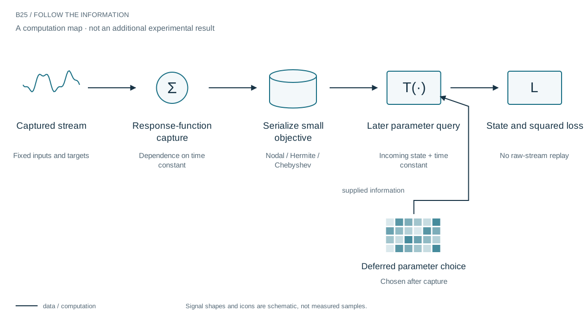
A block summary records how terminal state and squared loss depend on an incoming state and a still-undecided time constant. The observations enter three response functions. Their nodal values or value–derivative pairs are serialized, while timing supplies the remaining deterministic terms. The later query changes a parameter, not the captured target sequence.
This differs from storing the best-fit parameter: the recipient can revisit the objective over the retained domain. It also differs from retaining a waveform: it cannot answer an arbitrary historical question or introduce an unrelated nonlinear recurrence. The compact object is a program for a specified family of calculations.
Three functions replace a replay
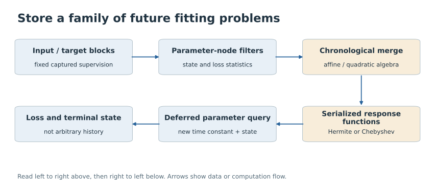
For a stable scalar filter, the final state is affine in its incoming state and squared error is quadratic. Three data-dependent functions of the time constant determine those quantities. They can be tabulated or interpolated during capture. Later queries evaluate the functions, not the original stream. This is a representation of a family of calculations, not a reconstructed waveform.
The target is fixed; the parameter is not
The permitted freedom matters. We can reconsider the filter time constant and incoming state while preserving the captured target sequence. We cannot invent new labels, add an arbitrary nonlinear recurrence, or ask where an unretained event occurred. The compact object is useful precisely when the application needs the questions it preserves.
A small object, with a strong ordinary rival
At equal storage, a 32-scalar-per-function Hermite representation passes all 108 record/version checks in the short panel, using 802 serialized bytes. So does Chebyshev interpolation—and Chebyshev is much more accurate. A natural cubic table needs the larger tested budget. Derivatives in the Hermite representation are charged as stored values, not treated as free information.
The stream can be longer than the memory
A separate million-sample panel restores a serialized checkpoint after every 1024 samples. Both Hermite and Chebyshev pass the prescribed terminal-state and mean-loss errors with 438-byte float32 objects. Computation still uses float64, and the process uses far more memory than the file. The experiment establishes a small retained objective, not a tiny complete runtime or unrestricted neural retraining.

A compact program for deferred learning
The long-stream result makes this vision tangible with small serialized objects and explicit error checks. Chebyshev interpolation is the strongest accuracy comparator in this panel, so the contribution is the retained objective and composition law rather than a compulsory spline implementation. Fast later queries must still repay encoding cost.
A different meaning of learning memory
A useful memory may preserve a choice rather than a picture of the past. Here, later parameter queries can be hundreds of times faster than replaying the declared scalar objective, after charging capture work. The broader opportunity is to identify important ML components with similarly small families of future questions. The hard boundary is information: a compact objective cannot answer questions it never encoded.
Evidence & further reading
The links below distinguish the project record from foundational literature. This revised story does not add a new application-validation experiment.
- Compression that preserves future computation. Spline research archive (2026). Local archive snapshot.
- Retunable objective memory: study 02 findings. Spline research archive (2026). Local archive snapshot.
- PASS-GLM: polynomial approximate sufficient statistics for scalable Bayesian GLM inference. Jonathan H. Huggins, Ryan P. Adams and Tamara Broderick (2017). Primary literature.