Instead of sending every sample, describe the instrument
Voiced speech combines an excitation with a changing acoustic filter. A compact model can send a description of the excitation and resonances, then synthesize sound at the receiver. This is the powerful classical intuition behind linear predictive speech coding. It also connects naturally to an operator toolbox: recurrences describe the dynamics, poles describe resonances, and a small state carries the response forward.
A filter model is not yet a transmitted format
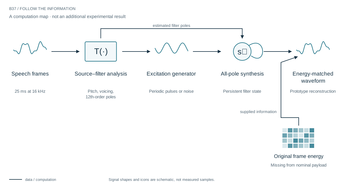
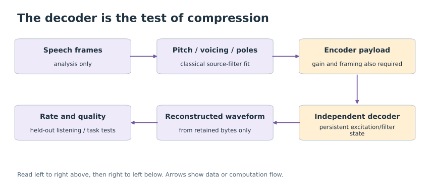
The analysis stage estimates voicing, pitch, and a resonant denominator. The synthesis stage needs excitation gain, persistent phase or noise conventions, filter state, and frame timing as well. A decoder separated from the original recording must obtain every one of those quantities from the encoded stream or a shared deterministic convention.
The prototype passes original voiced-frame energy directly to synthesis while omitting it from the nominal payload. It also assigns a bit rate without serializing and independently decoding quantized parameters. Those are not cosmetic bookkeeping problems: they mean the stated message is insufficient to run the decoder as measured.
A denominator becomes a sound model
Our prototype estimates a twelfth-order recurrence on 25-millisecond frames. A voiced frame gets a periodic excitation; an unvoiced frame gets noise. An all-pole filter shapes that excitation, and its state persists between frames. The model describes a family of signals rather than retaining all the original samples. This is established source–filter analysis, not a new result created by renaming LPC poles.
Stability is a useful piece of the puzzle
Multiplying coefficient j by gamma to power j contracts every pole by gamma. With gamma below one, a stable frame filter moves farther inside the unit circle. Four deterministic fixtures—silence, a tone, noise, and a harmonic pair—produce finite stable filters. The 150 Hz tone is estimated at 150.94 Hz because pitch is selected on an integer-lag grid. These checks establish a numerical pathway, not speech quality or stability under arbitrary switching.
The communication boundary revealed the missing information
The same-process synthesizer uses the original frame energy, but the stated voiced payload does not retain it. There is no serialized bitstream or independent decoder reload. The script’s nominal rate is assumed, not measured; thirteen full-precision coefficients alone would require 33,280 bits per second at the stated frame duration. That is an accounting example, not a lower bound on what a real quantized codec could achieve.
An audio model is not yet an audio codec
A related codebook experiment also learns and evaluates its filters on the same recording and passes pitch and gain without quantized transmission. Its spectral score cannot establish intelligibility. We therefore do not publish a fabricated listening comparison or a tiny bitrate headline. The paper gives the actual analysis and synthesis mechanism, stability checks, and the exact missing parts of the decoder interface.
Build the decoder before claiming the codec
The operator description remains useful for designing a compact generative signal model. A genuine ML codec contribution could learn residual codes, quantization, or a robust decoder, but must compare actual bytes and held-out quality. The present study preserves the classical prototype and explains precisely why its nominal low-rate claim is not established.
Where an ML contribution would have to live
A meaningful next contribution could learn an excitation model, an efficient quantized parameter space, or a task-specific sound representation. It would still need held-out speakers, complete bytes, and relevant perceptual or downstream tests. The useful lesson from this prototype is architectural: physical structure can make a representation small, but only a complete communication system can demonstrate compression.
Evidence & further reading
The links below distinguish the project record from foundational literature. This revised story does not add a new application-validation experiment.
- Source–filter vocoder v7: prototype implementation. Local speech project (2026). Local archive snapshot.
- Speech prototype automatic benchmark implementation. Local speech project (2026). Local archive snapshot.
- Cardinal Exponential Splines: Part I—Theory and Filtering Algorithms. Michael Unser and Thierry Blu (2005). Primary literature.