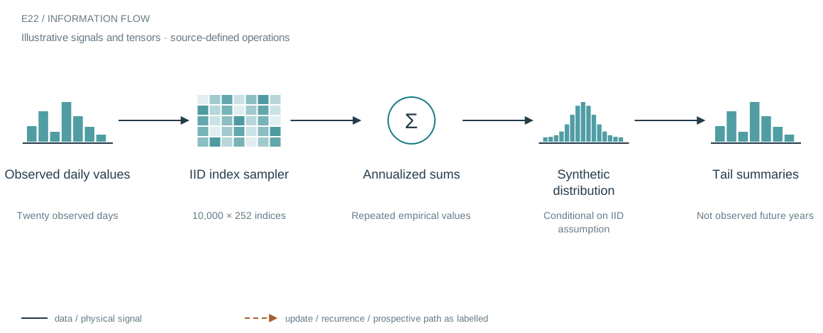
The architecture in context
What this comparison asks
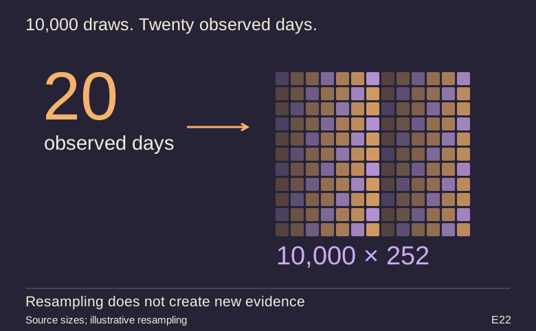
The notebook repeatedly samples daily values with replacement, adds 252 of them and summarizes the distribution of synthetic annual totals. This is a compact way to explore a specified resampling model. It is not a way to manufacture more independent market history or establish that future days follow the same distribution.
Who does what in the stack
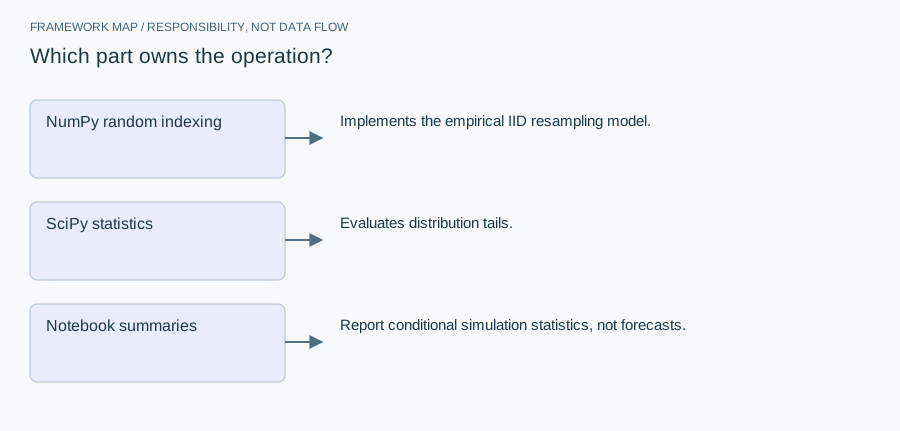
- NumPy random indexing
- Implements the empirical IID resampling model.
- SciPy statistics
- Evaluates distribution tails.
- Notebook summaries
- Report conditional simulation statistics, not forecasts.
NumPy makes the full simulation matrix explicit; SciPy supplies a t-distribution calculation elsewhere in the notebook. The engineering lesson is to label exactly what randomness was introduced. Repeated bootstrap draws reduce simulation noise conditional on the empirical sample, not uncertainty about whether that sample represents a new regime.
Open up the implementation
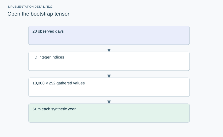
Open the bootstrap tensor
Resampling conditions on the empirical distribution of the observed days. More draws reduce Monte Carlo error in the synthetic quantiles but do not reduce uncertainty caused by an unrepresentative sample or serial dependence. The IID assumption is doing real work in the annual aggregation.
The mathematical contract
Blocked resampling may address some dependence, but choosing block length needs a defensible protocol and does not conjure missing regimes. The notebook’s absolute-value t-statistic in a directional tail calculation also requires correction before interpreting significance.
Implementation and resource card
- Capacity / budget
- 10,000 simulation rows are not 10,000 independent observed years. Memory is proportional to simulations × sampled days.
- Execution evidence
- This revision inspects and explains the archived implementation. It does not rerun the original workload. No unrecorded convergence time, throughput or accelerator result is supplied.
- Current reproduction context
- Current workstation, supplied by the author: Apple M4, 128 GB unified RAM, 40 GPU cores and 16 CPU cores. This is context for prospective reproduction, not attribution of every archived run. Python and framework versions are not fully locked for these historical sources; declarations, when available, are identified separately.
From explanation to a reproducible check
Use an all-negative sample and check that a directional profitability test does not return a misleading small positive-direction p-value. Distinguish a numerical simulation check from a test of the empirical assumptions.
Preserve input identities, configuration and failure records with the result. A successful numerical check only establishes the operation it exercises: it does not certify an entire dataset, model or deployed system. Reproduce the interface on a small deterministic input before optimizing throughput or increasing workload size.
A closer look at the implementation
The code that carries the idea
The index matrix has one row per simulation and one column per resampled day. Advanced indexing gathers observed values, then summing across columns produces a hypothetical year. The saved example uses only a small daily sample, so dependence and unobserved regimes dominate any interpretation of its tails.
    simulations = 10000
    sim_days = 252 # Trading days in a year

    # Generate random indices
    indices = np.random.randint(0, n, size=(simulations, sim_days))
    # Map indices to values
    bootstrapped_years = data[indices]
    # Sum each year
    yearly_pnls = np.sum(bootstrapped_years, axis=1)

    loss_prob = np.sum(yearly_pnls < 0) / simulations * 100
    worst_5_pct = np.percentile(yearly_pnls, 5)
    avg_yearly = np.mean(yearly_pnls)

    print(f"\n--- 2. BOOTSTRAP (1 year projection) ---")
    print(f"Avg Yearly PnL: {avg_yearly:.2f}")
    print(f"Prob of Loss:   {loss_prob:.2f}%")
Verbatim archive excerpt from analyze_significance.ipynb. Context-dependent historical code, not a standalone runnable program. Comments retain their original wording; the article distinguishes implemented behavior from stale or overbroad comments.
The boundary that matters
The separate t-test code uses the absolute t statistic with a one-tail survival function. That is not a valid directional positive-mean p-value for negative t. More generally, an IID bootstrap omits serial dependence; block resampling would be a different declared model, not a retroactive guarantee.