The architecture in context
What this comparison asks
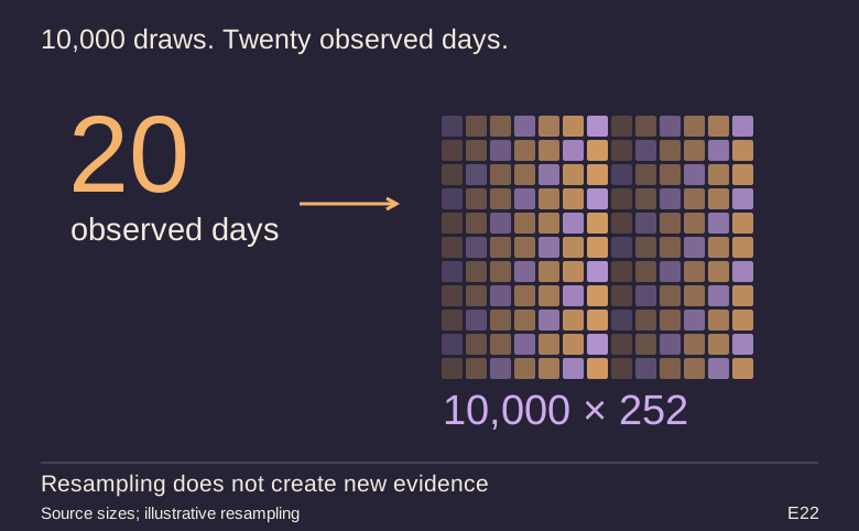
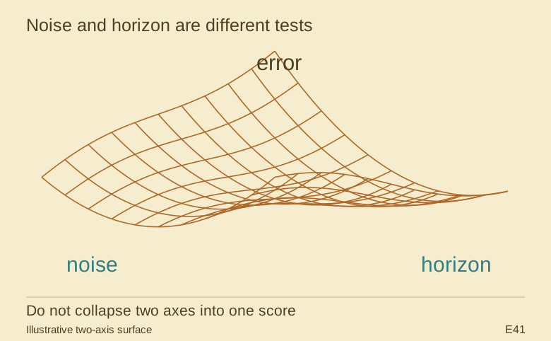
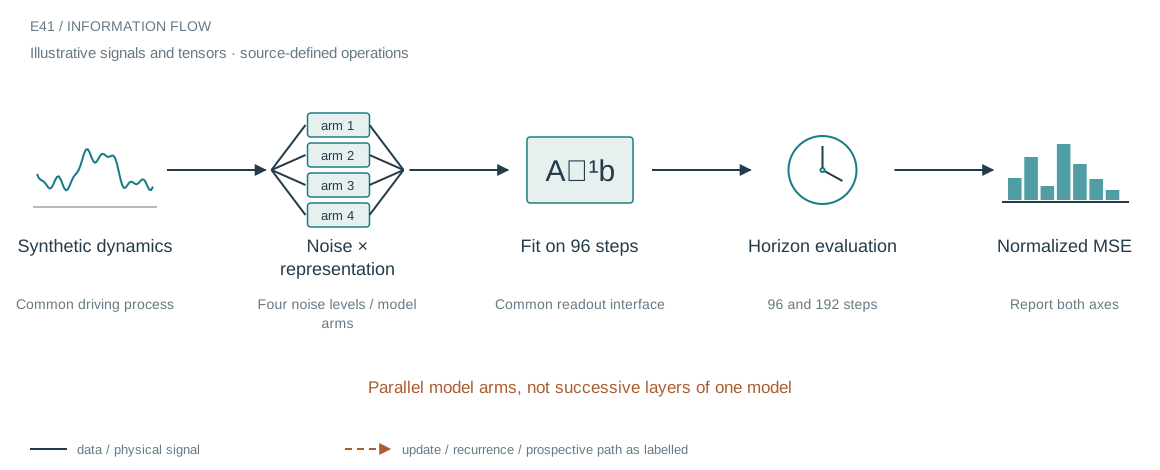
A recurrent model can work at its training horizon and drift later, or remain stable but fail under measurement noise. The archived panel varies both dimensions: training sequences have length 96, while the longer evaluation uses 192 steps; four noise levels and three seeds are retained. Many timesteps within one generated sequence are not independent replications.
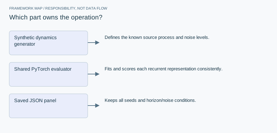
Who does what in the stack
- Synthetic dynamics generator
- Defines the known source process and noise levels.
- Shared PyTorch evaluator
- Fits and scores each recurrent representation consistently.
- Saved JSON panel
- Keeps all seeds and horizon/noise conditions.
The companion eval_arm function applies a shared ridge-readout interface to several pole choices. The saved metrics separate in-distribution and longer-horizon errors. A matched-pole reference has privileged structure and should be labeled as such rather than treated as an ordinary learned competitor.
From module map to executable structure
Inside Complex diagonal state-space model
This results or evaluation article shares the implementation in E40. The architecture below describes that companion, not a newly trained model.
Default 64 complex states, input 1/output 2, train length 96/test 192;1,500 training and 400 test sequences.
| Layer or branch | Output shape | Implementation detail |
|---|---|---|
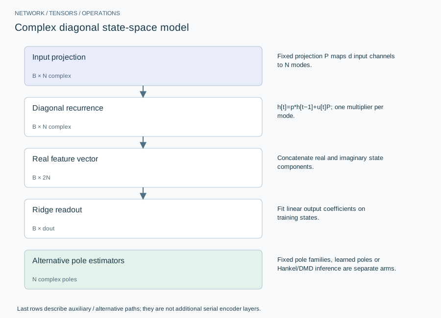
| Input projection | B × N complex | Fixed projection P maps d input channels to N modes. |
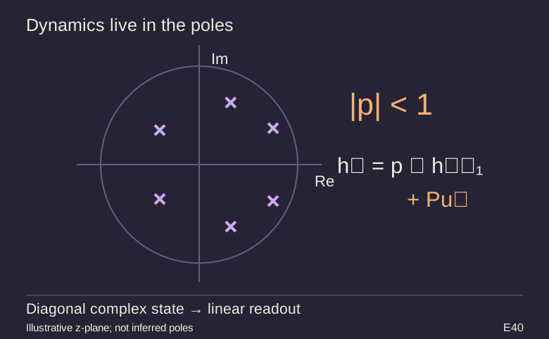
| Diagonal recurrence | B × N complex | h[t]=p*h[t−1]+u[t]P; one multiplier per mode. |
| Real feature vector | B × 2N | Concatenate real and imaginary state components. |
| Ridge readout | B × dout | Fit linear output coefficients on training states. |
| Alternative pole estimators | N complex poles | Fixed pole families, learned poles or Hankel/DMD inference are separate arms. |
The diagonal transition replaces a dense N×N state multiply with N elementwise products. Complex conjugate structure or real/imaginary expansion represents damped oscillation. A state model can be cheap to advance and still be poorly identified; pole radius, input projection and observability determine whether the output is useful.
The equation and the update
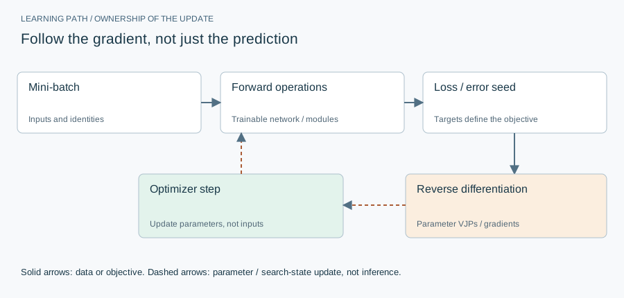
Default learned-pole arm 600 Adam steps at 5e-3; three seeds. DMD and fixed-pole arms do not use that optimizer budget. Known-system poles in a matched arm supply privileged information.
Implementation card / no invented benchmarks
Capacity, budget and execution evidence
- Parameters / retained state
- State is N complex values per sequence; readout width 2N before any bias convention. Pole-learning parameters are distinct from fixed projection and readout storage.
- Duration and hardware evidence
- No generic speedup is inferred from diagonal structure; training, identification and rollout need separate timings.
- Source coordinates
- E40 lines 65–155 and configuration 159–166; E41 metrics
- Current reproduction context
- Current workstation, supplied by the author: Apple M4, 128 GB unified RAM, 40 GPU cores and 16 CPU cores. This is context for prospective reproduction, not attribution of every archived run. Python and framework versions are not fully locked for these historical sources; declarations, when available, are identified separately.
Counts above are calculated from the stated layer shapes unless identified as saved measurements. They exclude optimizer state and nontrainable buffers. No archived training was rerun for this revision.
What these design choices change
Increasing N adds dynamical modes but may make the readout ill-conditioned. Longer Hankel windows change the identification problem, not just batch size. The source projects inferred eigenvalues inside radius .999; this avoids explosive autonomous modes but can bias nearly undamped dynamics.
Reproduction and measurement protocol
Check the impulse response of a single real pole and a conjugate pair against the recurrence. Reset state at sequence boundaries. Keep noisy observation targets separate from the clean reference used for evaluation, and report matched-pole arms as oracle-assisted rather than fully learned.
For a new run, save the resolved Python/framework versions, backend, dtype, seed, input shapes, batch size and exact source revision. Start with one batch and one update. Log training steps separately from epochs or environment steps. Do not equate the configured maximum with a completed budget or convergence.
Measure initialization/compilation, data preparation, warmed forward pass, training updates and evaluation separately. Synchronize accelerator work around timed regions using the chosen framework’s supported mechanism. Report peak process memory and framework allocation separately; parameter bytes exclude activations, gradients, optimizer state and input buffers. On a shared machine, begin with a single CPU worker and a small batch rather than claiming all available resources.
A closer look at the implementation
The code that carries the idea
The excerpt flattens batch/time features to fit W, then evaluates a fresh recurrent rollout and reports mean squared error divided by mean squared target magnitude. Because target noise contributes to both numerator and denominator, the metric’s interpretation changes with noise level.
def eval_arm(poles, P, utr, ytr, ute, yte, lam=1e-3):
    phi_tr = ssm_features(poles, utr, P).reshape(-1, 2 * poles.shape[0])
    W = ridge_fit(phi_tr, ytr.reshape(-1, ytr.shape[-1]), lam)
    phi_te = ssm_features(poles, ute, P).reshape(-1, 2 * poles.shape[0])
    pred = phi_te @ W
    err = ((pred - yte.reshape(-1, yte.shape[-1])) ** 2).mean() / (yte ** 2).mean()
    return float(err)                                                   # normalized MSE
Verbatim archive excerpt from closed_form_neat_osnr_ssm.py (companion source E40). Context-dependent historical code, not a standalone runnable program. Comments retain their original wording; the article distinguishes implemented behavior from stale or overbroad comments.
The boundary that matters
A single pooled mean can conceal which axis causes failure. The panel is a synthetic dynamics study, not a universal result for long-context sequence models. This article does not select a best noise regime after inspecting the record.