A fit is not an answer to every question
An inverse model is often judged by how closely it reproduces observations. But the quantity used downstream may be a derivative, a local stress, or another response that the observations barely constrain. Options provide a concrete example: accurate call prices do not automatically identify point gamma. This is a question about information, not solver precision.
The scale of the question is part of the answer
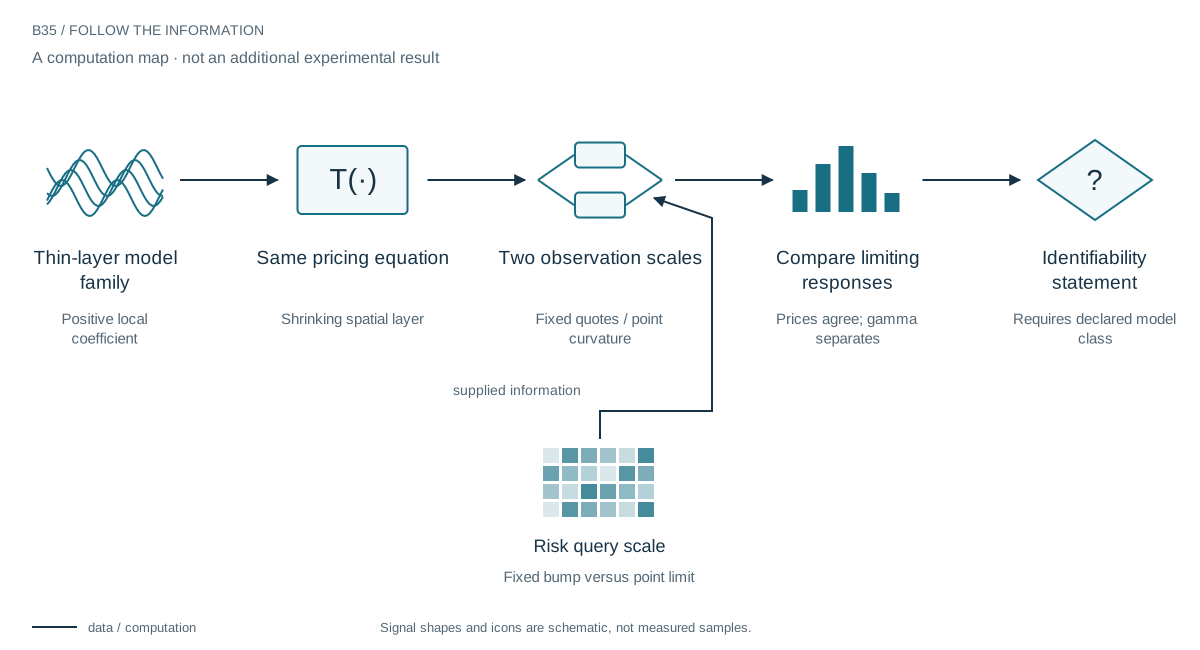
The thin-layer example changes a diffusion coefficient in an increasingly narrow neighborhood of the queried spot. Prices smooth over that neighborhood and converge to background prices. Point gamma remains sensitive to the local coefficient because the backward equation relates curvature to the maturity derivative there.
A fixed nonzero bump samples prices at separated locations and has a different limit. Letting the bump shrink first is not the same as letting the layer shrink first. This is why a tiny quote residual cannot alone establish a reliable point-risk estimate over an unrestricted family of thin layers.
Hide a different coefficient in a thin layer
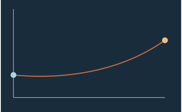
Our construction places one positive diffusion coefficient in a shrinking neighborhood of the spot and another outside it. At every fixed positive maturity, prices converge to the background prices. Point gamma at the center instead converges to the background gamma multiplied by the inverse coefficient ratio. Every nonzero layer has an ordinary constant-coefficient neighborhood, so this is not merely an ambiguous interface derivative.
Finite movements ask a different question
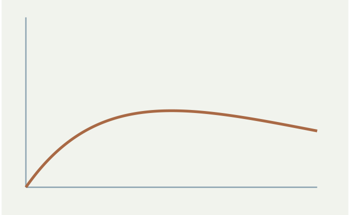
Hold a nonzero spot bump fixed and the finite-bump response converges to the background response. Let the bump go to zero first and the anomalous point curvature remains. The two limits do not commute. That distinction matters whenever a downstream decision treats an infinitesimal derivative as interchangeable with the response to an actual finite perturbation.

From an example to an information limit
For finitely many fixed quotes with fixed positive Gaussian noise, the thin-layer and background observation distributions become indistinguishable. Their point gammas remain separated. A uniformly reliable estimator of point gamma over this unrestricted family is therefore impossible. Minimum layer widths, stronger regularity, additional observations, or a different target change the problem; this is not a universal impossibility theorem for risk estimation.
Specify the scale of the risk question
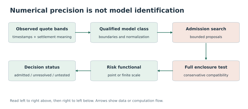
The practical lesson is to specify the spatial scale of a risk query and the regularity information supplied by the model class. Greater solver precision cannot replace that information. Finite responses may be more meaningful for some decisions, but their identifiability still requires its own observation argument.
What this contributes to learning
The lesson is to specify what must be identified before designing the representation or loss. A more expressive learned model can fit observations while introducing additional unconstrained responses. Operator analysis makes one such failure explicit and suggests choosing decision-relevant scales. It does not prove that finite-bump risk is identified from every sparse surface, nor that a trading application is ready.
Evidence & further reading
The links below distinguish the project record from foundational literature. This revised story does not add a new application-validation experiment.
- Compact computation and model ambiguity in option risk. Spline research archive (2026). Local archive snapshot.
- Compact, verifiable operator-based options risk. Spline research archive (2026). Local archive snapshot.