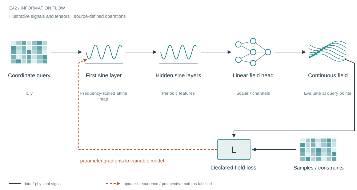
The architecture in context
The system we are building
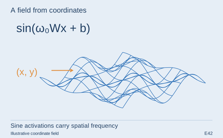
A coordinate network stores a field in its parameters and can be queried between training points. The archived SIREN implementation uses sine activations rather than a conventional ReLU stack. That makes frequency scale and initialization especially important: poorly scaled affine inputs can send both activations and derivatives into an unhelpful regime.
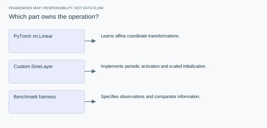
Who does what in the stack
- PyTorch nn.Linear
- Learns affine coordinate transformations.
- Custom SineLayer
- Implements periodic activation and scaled initialization.
- Benchmark harness
- Specifies observations and comparator information.
The project implements a SineLayer with separate first-layer and hidden-layer initialization, then uses it as a comparator for operator-based representations. SIREN is an established upstream architecture; the local contribution is a baseline implementation and the experiment around it.
From module map to executable structure
Inside SIREN coordinate baseline
2D coordinate input; width 64; first sine layer plus three additional sine layers; omega 0=30.
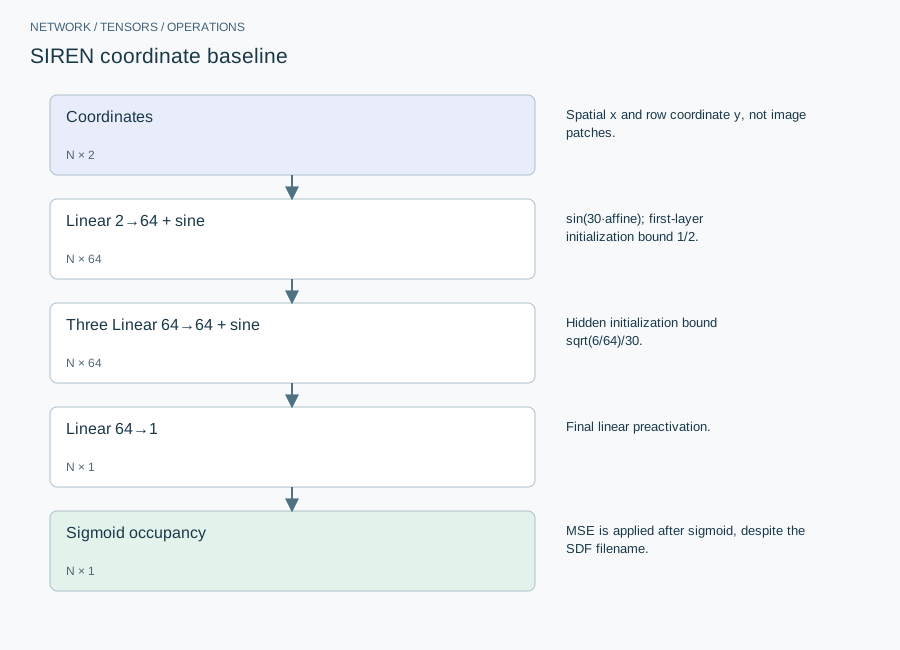
| Layer or branch | Output shape | Implementation detail |
|---|---|---|
| Coordinates | N × 2 | Spatial x and row coordinate y, not image patches. |
| Linear 2→64 + sine | N × 64 | sin(30·affine); first-layer initialization bound 1/2. |
| Three Linear 64→64 + sine | N × 64 | Hidden initialization bound sqrt(6/64)/30. |
| Linear 64→1 | N × 1 | Final linear preactivation. |
| Sigmoid occupancy | N × 1 | MSE is applied after sigmoid, despite the SDF filename. |
Sine activations carry high-frequency variations through a coordinate MLP. Their scale and initialization must be considered together: multiplying preactivations by 30 also scales derivatives. The final sigmoid bounds predictions but can saturate, reducing the gradient on confidently wrong occupancy values.
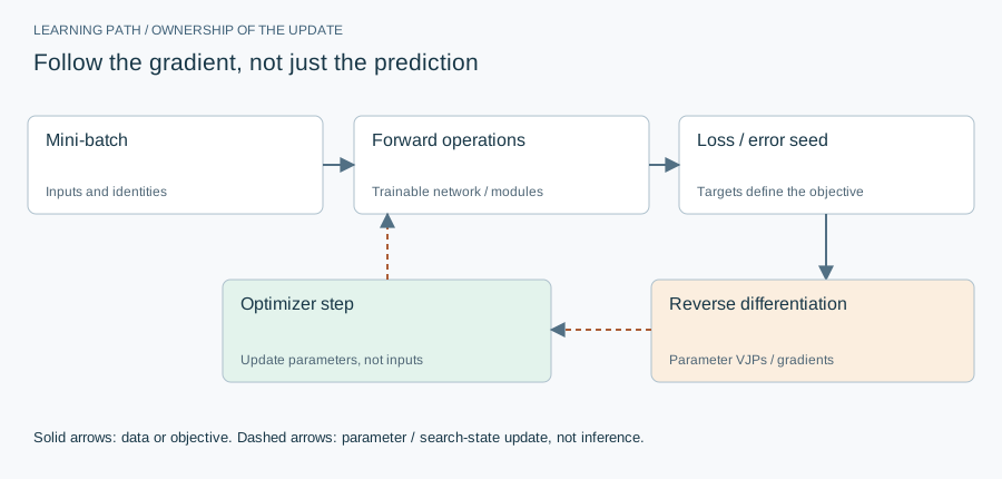
The equation and the update
Adam 1e-4, full coordinate batch, MSE(sigmoid(model(coords)), target); epoch count is a caller argument. The baseline fits sampled occupancy; the operator comparison receives exact innovation information.
Implementation card / no invented benchmarks
Capacity, budget and execution evidence
- Parameters / retained state
- 12,737 scalars including biases.
- Duration and hardware evidence
- The function measures training milliseconds, but this card does not substitute a new timing for an unidentified run.
- Source coordinates
- E42 lines 49–118
- Current reproduction context
- Current workstation, supplied by the author: Apple M4, 128 GB unified RAM, 40 GPU cores and 16 CPU cores. This is context for prospective reproduction, not attribution of every archived run. Python and framework versions are not fully locked for these historical sources; declarations, when available, are identified separately.
Counts above are calculated from the stated layer shapes unless identified as saved measurements. They exclude optimizer state and nontrainable buffers. No archived training was rerun for this revision.
What these design choices change
Width increases stored weights roughly quadratically in the hidden layers; more coordinates increase training activation memory without changing parameter count. Equal parameter count does not imply equal information access when one comparison arm receives exact edge innovations.
Reproduction and measurement protocol
Test coordinate normalization and the target’s meaning first. An occupancy discontinuity is not a signed distance function. Plot boundary localization as well as global MSE; a blurred edge can have reasonable average error while failing the geometric task.
For a new run, save the resolved Python/framework versions, backend, dtype, seed, input shapes, batch size and exact source revision. Start with one batch and one update. Log training steps separately from epochs or environment steps. Do not equate the configured maximum with a completed budget or convergence.
Measure initialization/compilation, data preparation, warmed forward pass, training updates and evaluation separately. Synchronize accelerator work around timed regions using the chosen framework’s supported mechanism. Report peak process memory and framework allocation separately; parameter bytes exclude activations, gradients, optimizer state and input buffers. On a shared machine, begin with a single CPU worker and a small batch rather than claiming all available resources.
A closer look at the implementation
The code that carries the idea
The excerpt initializes first-layer weights using the input width, while later layers include the frequency scale in the bound. Forward evaluation applies sine to a scaled affine transform. Reproducing only the sine activation while omitting these conventions would not reproduce this baseline.
class SineLayer(nn.Module):
    def __init__(self, in_features: int, out_features: int, omega0: float, is_first: bool = False) -> None:
        super().__init__()
        self.linear = nn.Linear(in_features, out_features)
        self.omega0 = float(omega0)
        self.is_first = bool(is_first)
        self.reset_parameters()

    def reset_parameters(self) -> None:
        with torch.no_grad():
            in_features = self.linear.weight.shape[1]
            if self.is_first:
                bound = 1.0 / in_features
            else:
                bound = np.sqrt(6.0 / in_features) / self.omega0
            self.linear.weight.uniform_(-bound, bound)
            self.linear.bias.uniform_(-bound, bound)

    def forward(self, x: torch.Tensor) -> torch.Tensor:
        return torch.sin(self.omega0 * self.linear(x))
Verbatim archive excerpt from compare_siren_sdf.py. Context-dependent historical code, not a standalone runnable program. Comments retain their original wording; the article distinguishes implemented behavior from stale or overbroad comments.
The boundary that matters
The surrounding comparison includes an operator reconstruction supplied with exact innovation moments. That is a different information interface from learning solely from point samples. Any speed or accuracy comparison must expose the cost and availability of those moments.