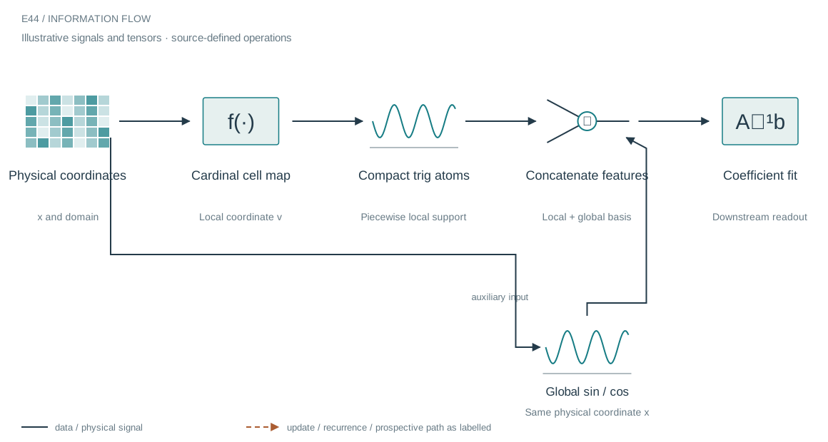
The architecture in context
The system we are building
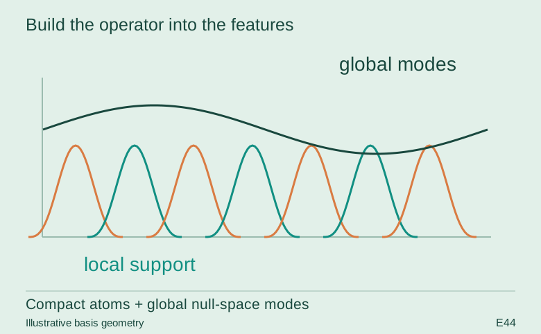
The layer converts coordinates into a dictionary rather than directly predicting a field. Local piecewise trigonometric atoms provide spatial degrees of freedom, while global sine and cosine functions represent the homogeneous oscillatory component. A downstream coefficient fit can use both through one tensor interface.
Who does what in the stack
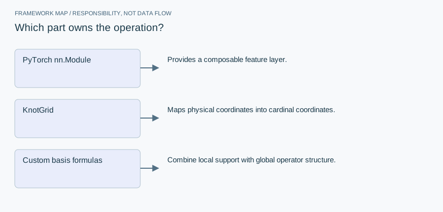
- PyTorch nn.Module
- Provides a composable feature layer.
- KnotGrid
- Maps physical coordinates into cardinal coordinates.
- Custom basis formulas
- Combine local support with global operator structure.
The custom nn.Module wraps grid construction, support masks and feature concatenation. The wavenumber is stored as a Python float in this implementation, so it is supplied configuration rather than a learned parameter. PyTorch integrates the resulting basis with the rest of a model.
Open up the implementation
Separate basis evaluation from coefficient learning
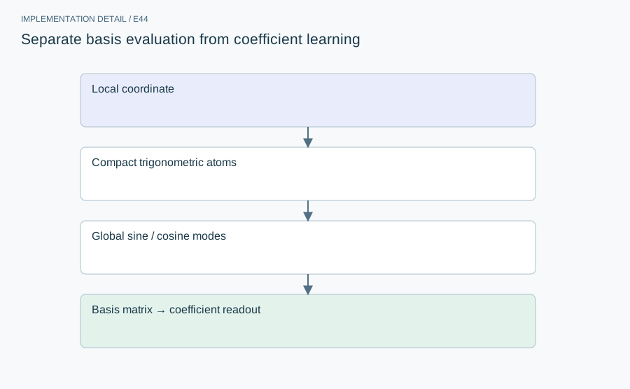
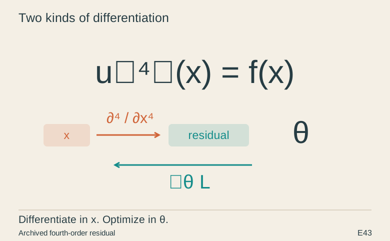
Local compact atoms describe representational degrees of freedom; the two global modes span a sinusoidal null space. A matrix of basis values can feed a learned or solved linear readout. Differentiating the global modes gives −k² times the mode, but that identity cannot be assigned to every local atom across its knots and boundaries.
The mathematical contract
Matching the basis to an operator can simplify a solve without creating a general neural PDE solver. Grid scaling, support endpoints and the k→0 limit are implementation concerns. The inspected formula divides by k, so zero frequency requires a separately derived limiting branch.
Implementation and resource card
- Capacity / budget
- The basis layer itself has no learned parameters in this source: k is a Python float. A separate coefficient vector has number_of_knots+2 entries.
- Execution evidence
- This revision inspects and explains the archived implementation. It does not rerun the original workload. No unrecorded convergence time, throughput or accelerator result is supplied.
- Current reproduction context
- Current workstation, supplied by the author: Apple M4, 128 GB unified RAM, 40 GPU cores and 16 CPU cores. This is context for prospective reproduction, not attribution of every archived run. Python and framework versions are not fully locked for these historical sources; declarations, when available, are identified separately.
From explanation to a reproducible check
Test support outside[0,2), continuity at knot boundaries and finite differences away from knots. Compare physical x with normalized local coordinates. Verify coefficient learning separately from the fixed basis module.
Preserve input identities, configuration and failure records with the result. A successful numerical check only establishes the operation it exercises: it does not certify an entire dataset, model or deployed system. Reproduce the interface on a small deterministic input before optimizing throughput or increasing workload size.
A closer look at the implementation
The code that carries the idea
The excerpt shows the optional global-nullspace branch being concatenated with local atoms. That branch uses physical coordinates directly; the local branch receives grid coordinates. Derivative scaling must therefore account for the coordinate map instead of applying one frequency convention everywhere.
    def forward(self, x: torch.Tensor) -> torch.Tensor:
        local_atoms = self.local_trig_spline(self.grid(x))
        if not self.include_nullspace:
            return local_atoms

        k = x.new_tensor(self.wavenumber)
        global_null = torch.cat([torch.sin(k * x), torch.cos(k * x)], dim=-1)
        return torch.cat([global_null, local_atoms], dim=-1)
Verbatim archive excerpt from steady_state.py. Context-dependent historical code, not a standalone runnable program. Comments retain their original wording; the article distinguishes implemented behavior from stale or overbroad comments.
The boundary that matters
The helper returning −k² times the field is valid for the appropriate homogeneous sine/cosine component, not an arbitrary combination of compact piecewise atoms across knots. The local formula also divides by k, so k=0 requires an explicit limiting implementation. These are reuse boundaries, not claims that every function in the file is production-ready.