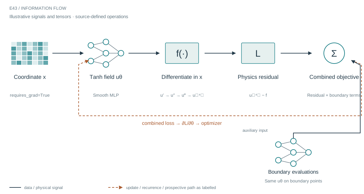
The architecture in context
The system we are building
A physics-informed network can be trained against a differential residual evaluated at collocation points. When that residual includes fourth derivatives, the derivative computation itself becomes a major part of the training graph. The archive implements this explicitly with repeated autograd calls over a tanh coordinate network.
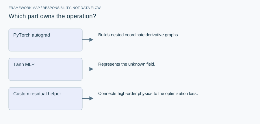
Who does what in the stack
- PyTorch autograd
- Builds nested coordinate derivative graphs.
- Tanh MLP
- Represents the unknown field.
- Custom residual helper
- Connects high-order physics to the optimization loss.
The custom helper constructs successive derivatives with create_graph enabled so the residual can still differentiate with respect to network parameters. PyTorch supplies the chain rule. The benchmark compares this training route with operator-aware alternatives under declared conditions.
From module map to executable structure
Inside Fourth-order physics-informed MLP
Scalar coordinate, four 32-unit tanh hidden layers, scalar field output.
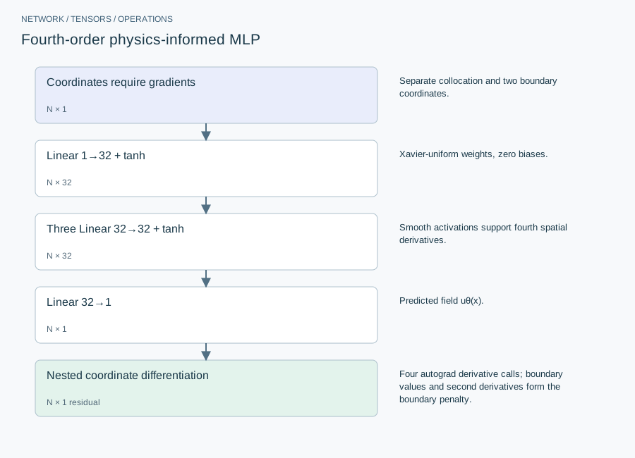
| Layer or branch | Output shape | Implementation detail |
|---|---|---|
| Coordinates require gradients | N × 1 | Separate collocation and two boundary coordinates. |
| Linear 1→32 + tanh | N × 32 | Xavier-uniform weights, zero biases. |
| Three Linear 32→32 + tanh | N × 32 | Smooth activations support fourth spatial derivatives. |
| Linear 32→1 | N × 1 | Predicted field uθ(x). |
| Nested coordinate differentiation | N × 1 residual | Four autograd derivative calls; boundary values and second derivatives form the boundary penalty. |
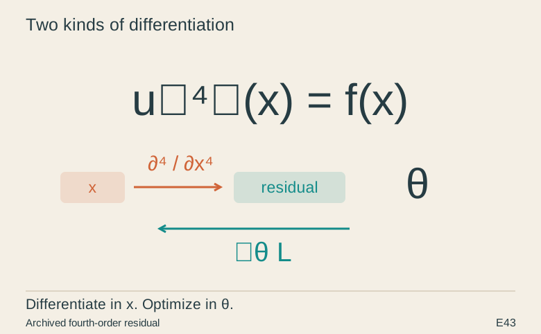
There are two different differentiation paths: derivatives with respect to x construct the PDE residual; derivatives of that loss with respect to network weights train the model. The coordinate graph must remain differentiable through all four derivative operations. ReLU would not be an equivalent activation for this strong-form fourth-order residual.
The equation and the update
Adam 2.5e-3; full collocation grid each epoch; loss=residual MSE+200×boundary penalty. Device selection in this script is CUDA if available, otherwise CPU—not MPS.
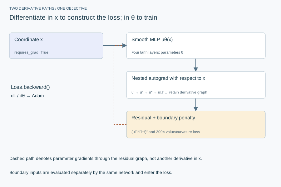
Implementation card / no invented benchmarks
Capacity, budget and execution evidence
- Parameters / retained state
- 3,265 trainable scalars; derivative graph storage is not included in that count.
- Duration and hardware evidence
- CPU fallback is intentional in the archived code. A proposed MPS port would need new operator-coverage and numerical checks.
- Source coordinates
- E43 lines 27–34, 41–58 and 93–129
- Current reproduction context
- Current workstation, supplied by the author: Apple M4, 128 GB unified RAM, 40 GPU cores and 16 CPU cores. This is context for prospective reproduction, not attribution of every archived run. Python and framework versions are not fully locked for these historical sources; declarations, when available, are identified separately.
Counts above are calculated from the stated layer shapes unless identified as saved measurements. They exclude optimizer state and nontrainable buffers. No archived training was rerun for this revision.
What these design choices change
The boundary weight 200 trades constraint enforcement against interior residual conditioning. A small parameter count does not make the nested derivative graph small. Increasing collocation points can increase memory and step time even though the architecture is unchanged.
Reproduction and measurement protocol
Before training, substitute an analytic polynomial into the derivative helper and compare its fourth derivative. Test boundary values and curvature separately. For memory, label the source’s CPU graph estimate as an estimate; it is not measured process RSS. Numerical error and memory should be compared at matched boundary and forcing conventions.
For a new run, save the resolved Python/framework versions, backend, dtype, seed, input shapes, batch size and exact source revision. Start with one batch and one update. Log training steps separately from epochs or environment steps. Do not equate the configured maximum with a completed budget or convergence.
Measure initialization/compilation, data preparation, warmed forward pass, training updates and evaluation separately. Synchronize accelerator work around timed regions using the chosen framework’s supported mechanism. Report peak process memory and framework allocation separately; parameter bytes exclude activations, gradients, optimizer state and input buffers. On a shared machine, begin with a single CPU worker and a small batch rather than claiming all available resources.
A closer look at the implementation
The code that carries the idea
The excerpt repeatedly asks for a coordinate gradient using a ones-like output seed. For a pointwise scalar-output network evaluated independently at each coordinate, this gives the desired per-point derivative. Cross-sample coupling would require revisiting that assumption.
def fourth_derivative(y: torch.Tensor, x: torch.Tensor) -> torch.Tensor:
    dy = torch.autograd.grad(y, x, torch.ones_like(y), create_graph=True, retain_graph=True)[0]
    dyy = torch.autograd.grad(dy, x, torch.ones_like(dy), create_graph=True, retain_graph=True)[0]
    dyyy = torch.autograd.grad(dyy, x, torch.ones_like(dyy), create_graph=True, retain_graph=True)[0]
    dyyyy = torch.autograd.grad(dyyy, x, torch.ones_like(dyyy), create_graph=True, retain_graph=True)[0]
    return dyyyy
Verbatim archive excerpt from compare_classic_pinn.py. Context-dependent historical code, not a standalone runnable program. Comments retain their original wording; the article distinguishes implemented behavior from stale or overbroad comments.
The boundary that matters
A memory estimate derived from parameter or activation counts is not measured peak process or device memory. Automatic differentiation is exact for the represented computational graph up to numerical arithmetic; it does not make the fitted field or PDE solution exact.