42 stories · 42 visual directions

Explore the ideas.

Fields, physical systems, measured images and model memory. Each illustration links to the research story and its technical manuscript. Controls are manual by default. Captions distinguish recorded results from explanatory examples.

B01 · When physics learning needs a solve, not a training loop ↗
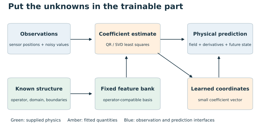
Sensor values and known physics feed a fixed feature bank and coefficient estimator, producing predictions.
Actual module structure of the fixed-basis studies. Supplied physics and learned coordinates have different roles; this is not a trained deep network.

B02 · 4.2× faster spline-layer evaluation through cardinal structure ↗

EXPLORE THE IDEA

Four taps, not a full grid

The measured gain appears when the grid gets large.

LOCAL SUPPORTOne query touches four coefficients32 shown · 512 stored per edgeActive location changes; support size does notARCHIVED MPS FORWARD PASSLarge-grid measurementDense explicit cardinal5.435 msStreamed local taps1.286 ms4.23×at this workloadSmall-grid losses remain in the result chart
50%
The coefficient-strip interaction is schematic. The 512-coefficient forward timings, 5.435 ms dense and 1.286 ms streamed, are archived MPS measurements for batch 1024, 32 inputs and 64 outputs. The smaller-grid route can lose; the full result plot below retains that crossover.

B03 · Exact smoothness losses for spline networks—without sampling the integral ↗

EXPLORE THE IDEA

An integral becomes geometry

The same continuous curvature, written in coordinates.

THE CONTINUOUS OBJECTA neural response between samplesCurvature energy 4.303THE COEFFICIENT OBJECTOnly overlapping supports interactQ is computed; its corner bands are periodic
50%
Computed periodic cubic curvature Gram for eight basis functions, integrated with four-point Gauss quadrature per cell (exact for these products up to rounding). The curve and quadratic energy use the displayed Gram matrix. Unit cell spacing; not a neural training-speed benchmark.

B04 · Grow a spline network without disrupting its predictions ↗
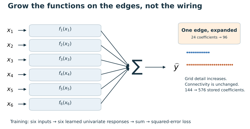
Six inputs pass through six spline edges and a summation. Each edge expands from 24 to 96 coefficients.
Actual six-edge additive architecture. Refinement changes edge resolution, not connectivity. Inset dots schematically indicate grid density.

B05 · Build boundary conditions into a learned model instead of penalizing them ↗

EXPLORE THE IDEA

Change the path, keep the boundary

An editable waypoint with fixed endpoint positions and tangents.

CONSTRAINED TRAJECTORYMove the waypoint, not the endpointsFIXED BOUNDARY DATAPosition and tangent stay attachedLEFTy = 0.20y′ = 0.36RIGHTy = 0.40y′ = −0.24Interior y = 0.50Two C¹-connected cubic Hermite cells
50%
Two computed cubic Hermite cells share an interior value and derivative. The slider changes that value; both outer values and outer derivatives remain fixed. This illustrates a parameterization, not an optimized physical trajectory.

B06 · Beyond a direct KAN: learning the physical law that extrapolates ↗

EXPLORE THE IDEA

Learn the missing law

Known transport and diffusion surround one unknown response.

A FIELD EVOLVESKnown conservation structureuₜ = νuₓₓ − ∂ₓF(u)LEARN THIS COMPONENTThe constitutive response FState range ±1.35Flux is computed; field is schematic
50%
The colored x–t field is an analytic schematic, not a PDE rollout. The flux plot evaluates F(u)=u²/2+0.08 sin(4u). The learned-versus-direct comparisons below are archived experiments; the flux dictionary contains this generating component.

B07 · Learning physical laws from noisy data without differentiating the noise ↗

EXPLORE THE IDEA

Integrate through the noise

A local window asks a better-conditioned question.

OBSERVATIONSA window moves across noisy samplesAN INTEGRATED QUESTIONWeighted average in the window-0.332from 24 contributing samples∑ wᵢ yᵢ / ∑ wᵢSynthetic observations; no fitted uncertainty
50%
Deterministic synthetic noisy samples and a compact cosine test window. The readout is their normalized weighted average, not an estimated physical law or a denoising-accuracy result.

B08 · Learning aircraft vibrations with a compact dynamical model ↗

EXPLORE THE IDEA

Listen to a structure

A ground-vibration test, not an autonomous flight.
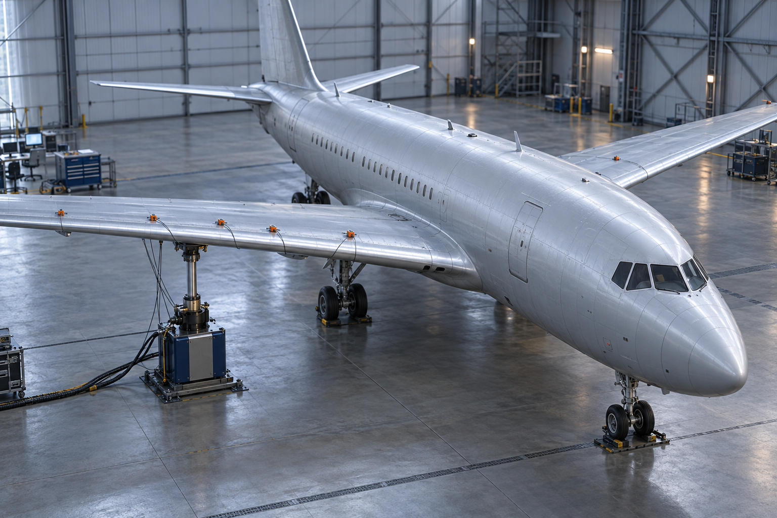
AI-generated editorial physical contextEditorial illustration
SENSOR RESPONSEA compact dynamical carrierStable poles · learned readout
50%
AI-generated editorial ground-test scene. The animated sensor channel is a computed damped sinusoid, not a recorded aircraft trace or deformation. The benchmark results discussed below remain separate.

B09 · Better coordinates or a bigger network? ↗

EXPLORE THE IDEA

One position. Two futures.

Velocity separates states that a snapshot merges.

POSITION VIEWEqual now does not mean equal nextv = +1v = −1Time from crossing 0.00STATE VIEWPosition × velocitypositionvelocityThe two trajectories remain distinct in state
50%
Computed free-motion example: x₁(t)=t and x₂(t)=−t. The position view merges the two at t=0; the phase portrait keeps their velocities distinct. No measured robot data is implied.

B10 · How small can a learned drone model become? ↗

EXPLORE THE IDEA

A smaller onboard model

Program size and prediction quality are different axes.
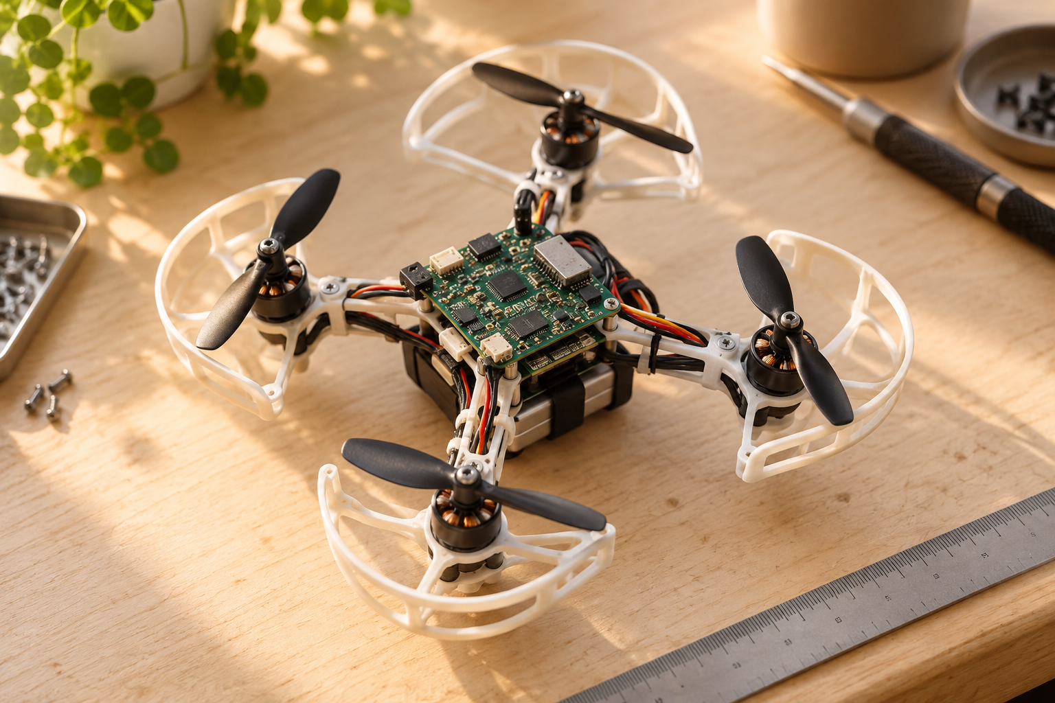
AI-generated editorial physical contextEditorial illustration
RETAINED PROGRAMSmall is a resource result24,288bytes · compact program≈24.79 MBsource + adapted neural programsNeural ensemble wins predictive accuracy
50%
AI-generated editorial nano-drone. Sizes are archived retained-program counts: 24,288 bytes compact versus approximately 24.79 MB for source-plus-adapted neural programs. They are not total process memory. The adapted ensemble was more accurate. The reveal is not a flight replay.

B11 · Continual learning without a replay buffer: what can we actually guarantee? ↗

EXPLORE THE IDEA

Keep every observation. Still change your mind.

Objective preservation is not behavioral preservation.

EVIDENCE LEDGERBoth targets remain in memoryEarlier observationtarget +1 · weight 1Later observationtarget −1 · weight 0.50MODEL STATEA changed optimumc* = 0.200Old squared error0.640No observation was erased
50%
Exact scalar ridge example with λ=1: target +1 receives weight one and target −1 receives the slider weight w. The optimum is (1−w)/(2+w). Old squared error changes even though no evidence is discarded.

B12 · Zero forgetting where it can be guaranteed ↗

EXPLORE THE IDEA

A region learning cannot touch

The update has support outside the protected interval.

A SUPPORT MASK, NOT A REPLAY BUFFERFreeze every support touching the regionPROTECTED INPUTSLocked coefficientsFree supportSchematic mask; fixed basis and coordinatesTHE REPRESENTED FUNCTIONThe old and new curves coincide hereComputed local update · protected interval unchanged
50%
Computed compact cubic B-spline update on a fixed coordinate system. Its support is entirely to the right of the protected region; the left-hand field and curve stay unchanged. Not a general neural-network zero-forgetting guarantee.

B13 · Version control for learned models: commit, roll back and forget explicitly ↗

EXPLORE THE IDEA

Review the change before it becomes the model

A model update with an explicit commit boundary.

MODEL / response-lawA reviewable changeparent v001+ local correction at x = 0.76 protected interval unchangedCOMMITInterface concept, not a production logCURRENT / CANDIDATEAcceptance is a separate operationCommitted: v002
50%
Interactive design sketch of propose, validate, commit and reject states. Curves are computed illustrations; displayed decisions are not logs or a shipped version-control product.

B14 · Can a frozen encoder keep learning new classes? ↗

EXPLORE THE IDEA

Expensive perception. Small adaptation.

Count what the frozen representation already contributes.

FROZEN REPRESENTATIONPerception does not start from zeroDINOv2 ViT-B featuresThe encoder stays fixed; only the readout changesARCHIVED CIFAR-100 PANELWhat does the readout add?88.47%ordinary linear ridge89.10%cosine-expanded ridge+0.63 percentage points in this panel
50%
Actual archived final CIFAR-100 accuracies: linear ridge 88.47%, cosine-expanded ridge 89.10%, on the named frozen DINOv2 features. The graphic reveals the incremental difference; it does not fabricate source images or a confusion matrix.

B15 · Evolve the network; solve the readout ↗

EXPLORE THE IDEA

Search the graph. Solve the readout.

Different structures, the same conditional linear problem.

OUTER SEARCHCandidate 3 / illustrative topologyINNER SOLVEFit the output, conditional on the graphZ(graph)↓(ZᵀZ + λI) W = ZᵀYTopology illustrated; output fitting is conditional
50%
Four illustrative graph candidates, not saved evolutionary champions. The parity construction counts in the article are separate archived results. The animation changes topology without inventing a fitness improvement.

B16 · Is your “local learning” algorithm actually backpropagation? ↗

EXPLORE THE IDEA

Follow the error signal

Local software blocks can still implement the global chain rule.

REVERSE-MODE SWEEPSame chain rule, separate blocksJ1J2J3J4J5←←←←Error travels backward through every blockTHE LOCAL OPERATIONAn adjoint is not a new learning ruleδℓ₋₁ = Jℓᵀ δℓCurrent block: 3Packaging ≠ differentiation ruleFinite relaxation is a separate algorithm
50%
Illustrative adjoint propagation δ at one block at a time. The direction and Jacobian-transpose operation describe reverse-mode differentiation, not biological activity or a gradient-free learner.

B17 · Learning between events instead of stepping through time ↗

EXPLORE THE IDEA

Nothing arrives. The state still evolves.

An event is not the same thing as a simulation time step.

EVENT ARRIVALSThree impulses, continuous evolutionBETWEEN EVENTSEvaluate the state directlyz(t) = 0.683ż = −7zz(t + Δ) = exp(−7Δ) z(t)Until the next impulse changes the state
50%
Computed linear exponential responses to three specified impulses. The cursor reveals the exact state between arrivals; event positions are synthetic and do not represent a recorded spiking network.

B18 · The same memory dynamics, different results at low precision ↗

EXPLORE THE IDEA

Rounding has a coordinate system

Rotate the lattice, change the decoded answer.

DECODED LATTICEA coordinate choice affects roundingBlue: original · copper: rounded and decodedSAME UNROUNDED STATEDifferent finite-precision answerRotation 45°(0.707, 0.354)Error 0.0882Step 0.25 in the rotated coordinates
50%
Computed rounding of the fixed point (0.62,0.34) on a lattice of step 0.25, after rotating coordinates. Both the lattice and decoded point are calculated. This geometric example is not an archived low-precision memory trajectory.

B19 · Update a robot’s dynamics model without rewriting its entire memory ↗
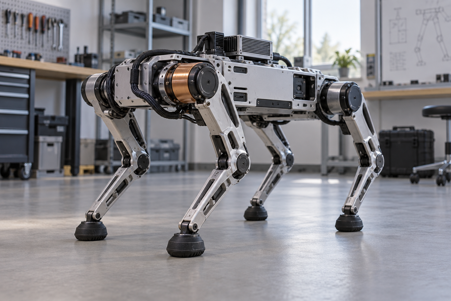
Editorial 3D rendering of a mechanically plausible quadruped robot in a laboratory; the near hip has a copper actuator casingLOCAL MODEL MAINTENANCEAn actuator response changes
REPAIR A MODEL, NOT ITS HISTORY

Let one part change.
Keep the rest intact.

A local coefficient update changes a chosen response region. Protected behavior stays on the original curve.

protectedinput →response

— proposed response · ··· original

Mechanism illustration, not a measured actuator trace. Preserving this curve is not a robot-safety guarantee.

65%
AI-generated editorial robot rendering with an analytically computed, synthetic local-update overlay. The archived control experiment used HalfCheetah-v5 simulation—not the pictured quadruped or a physical laboratory trial. The curve illustrates local response preservation; the separate admission calculation and closed-loop results are explained below.

B20 · Why a better dynamics model can still produce a worse controller ↗

EXPLORE THE IDEA

The feedback loop is the test

A nearly correct inverse did not deliver full recovery.

COMPOUND-LAG RESTORATIONSame frozen actor, fresh actuator lawsShared-prior fit0.8966Supplied true inverse0.8977PREDECLARED TARGETThe full recovery gate still failed0.90restoration thresholdA better model is notautomatically a better controller.The true inverse is not an optimal-policy ceiling
50%
Actual compound-lag restoration summaries: shared prior 0.8966; supplied true inverse 0.8977; predeclared target 0.90. These are aggregate archived results with the same frozen actor, not a simulated rollout video or an optimal-control bound.

B21 · Your physics loss went down. Did your predictions improve? ↗

EXPLORE THE IDEA

A field is not a trajectory

A harmless-looking drift changes where the particle ends up.

TWO VELOCITY FIELDSBoth are exactly divergence-freeDOWNSTREAM QUESTIONWhere does the particle arrive?∇ · v₁ = ∇ · v₂ = 0Separation 0.100A residual cannot choose the drift.Synthetic constant-field counterexample
50%
Computed counterexample: two constant velocity fields (1,0) and (1,0.2) both have zero divergence, but their particle trajectories separate. This is not a replay of the measured turbulence experiment.

B22 · Discard the measurements, change the prior, reconstruct again ↗

A retained quadratic objective supports a changed reconstruction priorMeasured samples become a fixed data term. That term branches to a smoothness prior and a total-variation prior within a shared coefficient space.REUSABLE INFERENCE INTERFACEmeasured samples½cᵀGc − bᵀcsmoothness priorTV priorthe data term stays fixed; the reconstruction choice changes
Illustrative information-flow map. The archived CT experiment keeps the measured scan inside the article; this cover distinguishes the reusable-objective idea from the separate reconstruction comparison.

B23 · A real CT scan tests our compression idea ↗

INSIDE THE EXPERIMENT

One scan. Different ways to remember it.

Drag the divider to inspect the reconstructions from the same measured acquisitions.

Walnut slice reconstructed from eight-bit raw measurements with total variation Same walnut slice reconstructed from cardinal-spline statistics Cardinal splineRaw + TV

MEASURED FAN-BEAM CT · 2D

What survives compression?

The shell, internal folds and reconstruction artifacts are data—not a drawing of a scanner.

Cardinal spline
6.31% view error 14,100 message bytes
Eight-bit raw + TV
4.23% view error 7,608 message bytes

Errors predict development projections, not image ground truth. Numeric message sizes exclude shared infrastructure.

50% compact / 50% raw
Actual archived 82 × 82 reconstructions, shown at their native information resolution with the same linear grayscale window; no AI enhancement. Images are from the original admission comparison, not the later matched-TV diagnostic. The slice is not a 3D volume or a patient scan. Data: Hämäläinen et al., Tomographic X-ray data of a walnut, CC BY 4.0. Reconstruction and display: this project. No reserved measurements were read for this figure.

B24 · Why sharing models is not enough for collective intelligence ↗

EXPLORE THE IDEA

Sharing cannot supply a missing distinction

A joint mission needs more than compatible messages.

A JOINT MISSIONVisit, avoid, then inspect in orderABSHARED STATEA message cannot invent experienceVisit learnedAvoid learnedInspection A learnedInspection B missingConceptual map; no physical swarm result
50%
Illustrative grid mission with visit, avoid and ordered inspection states. The missing second-inspection state is explicitly marked; no physical swarm footage or successful collective capability is fabricated.

B25 · Keep the loss function, discard the training stream ↗

EXPLORE THE IDEA

Remember the question, not every sample

A stream becomes a surface of future objective values.

OBSERVED STREAMOne set of samples, many later questionsSynthetic data generated by a damped responseOBJECTIVE AS A FUNCTIONQuery a time constant after acquisitionτ = 1.00 · loss = 0.1074
50%
Computed toy objective for a damped exponential with a variable time constant. The visible data and loss curve are generated from the same deterministic samples. It explains objective retention; measured compression results remain below.

B26 · Merge learning histories without repeatedly recompressing them ↗

EXPLORE THE IDEA

Merge without another approximation

Fixed parameter nodes survive an order-preserving tree.

CHRONOLOGICAL BLOCKSRetain the same parameter nodes01121023120324104123Block values add component by component.MERGE RESULTParenthesization does not resample(A + B) + (C + D)A + (B + (C + D))Both give [7, 9, 7]Time order remains part of the state contract
50%
Illustrative three-node vectors from four chronological blocks. Their component-wise sum is identical under the two displayed parenthesizations. This does not permit rearranging time-dependent state transitions.

B27 · Recalibrate a physical model after the raw data is gone ↗

EXPLORE THE IDEA

Calibration can happen later

Retain the quantities needed by a declared physical model.
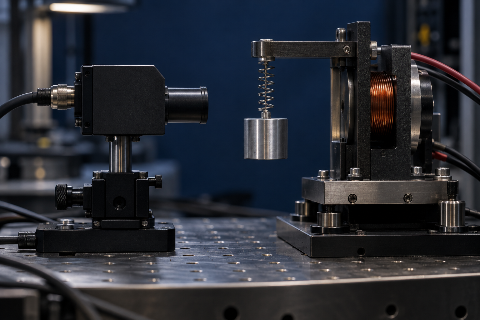
AI-generated editorial physical contextEditorial illustration
LATER MODEL QUERYA changed calibration parameterCandidate frequency 2.00Computed illustration; no new measurements
50%
AI-generated editorial oscillator bench with a computed candidate sinusoid. The slider changes frequency, not experimental calibration evidence. The retained-products mechanism and archived physical-memory results appear below.

B28 · How long can compressed memory remain trustworthy? ↗

EXPLORE THE IDEA

A precise answer can still be refused

A numerical uncertainty budget is part of the interface.

THE NUMERICAL ANSWEREstimate plus an explicit allowance0.500 ± 0.030Gray region: the requested precision budgetTHE APPLICATION REQUESTIs this enclosure narrow enough?Tolerance 0.052ACCEPTSynthetic fixed allowance, not empirical coverage
50%
Synthetic query: estimated response 0.5 with a fixed numerical allowance 0.03. The control changes the requested tolerance and therefore acceptance. This is an exact toy decision, not a fitted trajectory through archived checkpoints.

B29 · Can dynamical models shrink a transformer’s KV cache? ↗

EXPLORE THE IDEA

Tiny key error. A different answer.

The future query determines what compression must preserve.

KEY RECONSTRUCTIONError can become almost invisibleε = 3.16e-4k₁ = (1, +ε)k₂ = (1, −ε)q = (0, 1/ε)ATTENTION OUTPUTThe query amplifies the lost directionOriginal keys0.7616Both keys collapsed0Output error stays tanh(1); query norm grows
50%
Computed two-key counterexample: keys (1,±ε), values ±1, query (0,1/ε). Replacing both keys with (1,0) drives key error to zero while attention-output error remains tanh(1). Query norm grows; typical-model behavior is not implied.

B30 · A physics solver that computes at interfaces instead of everywhere ↗

EXPLORE THE IDEA

Solve the interior once

A continuous cell can communicate through its endpoints.

EXACT CELL INTERIORTwo endpoint values determine the field−u″ + 4u = 0GLOBAL INTERFACE CHAINThe interior unknowns disappearBalance outward derivatives at interfaces.Sources require their own cell load
50%
Computed source-free solution of −u″+qu=0 in a single cell, with q=4 and a variable right endpoint. Neighboring cells are a schematic interface chain; they do not form a recorded pricing solve.

B31 · Why exponential models become numerically unstable—and how to fix it ↗

EXPLORE THE IDEA

Two modes become one derivative

A finite limit deserves stable coordinates.

COLLIDING POLESThe function has a finite limitStable divided difference across t ∈ [0,2]BINARY64 CALCULATION AT t = 1Close roots expose cancellationPole gap 3.16e-9expm1: 0.3678794418subtract: 0.3678794375limit: 0.3678794412Actual arithmetic, not a timing animation
50%
Computed exponential divided difference versus its derivative limit at t=1, α=−1. The stable value uses expm1; the expanded value uses subtraction in JavaScript binary64. This is a numerical illustration, not a timing benchmark.

B32 · A useful numerical service on one CPU thread ↗

EXPLORE THE IDEA

A whole service on one thread

Request, calculation, enclosure, response.

NATIVE SERVICE / REPLAYA complete request has a complete cost01 parse supplied field02 assemble exact cells03 enclose 23 prices + 2 responses04 serialize outputARCHIVED ONE-THREAD MEASUREMENTApple M4 Max · shared host4.793 mswarm median · complete service2.219 MiBpeak native-process memoryNot a live monitor or low-power-device test
50%
Interface replay of the documented native-service contract, not a live request or screen recording. Reported 4.793 ms warm median and 2.219 MiB peak native memory are archived Apple M4 Max measurements, not edge-device or hard-real-time claims.

B33 · Return an error bound with the prediction ↗

EXPLORE THE IDEA

Preserve the cancellation

The quantity you ask for has its own error geometry.

SIGNED READOUTTwo nearby requests can cancelCopper minus blue: the combined questionCOMBINE BEFORE TAKING A NORMDo not discard useful cancellationSigned L² norm 0.4676Illustrative L² geometry, not the certified bound
50%
Computed signed Gaussian readout example: two unit-height bumps approach and cancel. The displayed signed L² norm is obtained by numerical integration of the illustrated functions; it is not the paper’s certified Green-kernel bound.

B34 · Don’t trust the model’s warning—verify it independently ↗

EXPLORE THE IDEA

Trust the check, not the search

A concrete witness crosses a narrow verification boundary.

UNTRUSTED PROPOSERSend fields, not claimed risk numbersmodel θ₁model θ₂Fields here are schematicINDEPENDENT RECIPIENTRecompute each claimed propertyRequest bindingParameter validityObservation compatibilityResponse separationIllustrated checks are not live security results
50%
Protocol illustration: validate a request-bound pair of model fields, recompute observation compatibility, and check response separation. Status transitions illustrate the protocol; they are not live parser logs or market certification.

B35 · Two models fit the data. Can they still disagree about risk? ↗

EXPLORE THE IDEA

Prices agree. Local curvature need not.

A thin layer makes the scale of the question visible.

COEFFICIENT FIELDA thinner and thinner local layerbackground a₀ε = 0.0379DIFFERENT LIMITING QUESTIONSFor a₁ = 2a₀Price gap → 0Point gamma → ½ Γ₀Finite bump ≠ infinitesimal curvatureLimits stated analytically; no invented prices
50%
Illustration of a shrinking coefficient layer. Readouts state the analytical limiting relation for a₁=2a₀: the price difference tends to zero while point gamma tends to half the background value. The drawing does not fabricate a finite-width price solution.

B36 · When a fast, accurate model fails on real data ↗

EXPLORE THE IDEA

A working engine. A closed application gate.

Optimizer success is not observation compatibility.

ALL PROPOSAL FAMILIESNo candidate crossed the gateHomogeneous12Clock-study midpoints60Direct feasibility20ADMISSION RESULT0 accepted92 proposals20 overlapping views120 risk directionsremained untestedOptimizer success does not imply admission
50%
Actual archive counts: 12 homogeneous, 60 clock-study and 20 direct-feasibility proposals; none admitted. Twenty overlapping views are not independent trials. The downstream 120 risk directions remained untested.

B37 · How much speech can a tiny dynamical model preserve? ↗

EXPLORE THE IDEA

A sound is a source through a filter

Change the resonance, not a decorative waveform.

SOURCE–FILTER SPECTRUMHarmonics shaped by resonancesGenerated spectral envelopes, not a recordingTIME–FREQUENCY VIEWA synthetic formant sweepMove the cursor to inspect a formant position
50%
Computed synthetic source–filter spectral illustration, not recorded speech, a listening test or a measured codec rate. Harmonic excitation and two resonance envelopes are explicitly generated; no audio plays.

B38 · Can a laptop hear you breathe? ↗

EXPLORE THE IDEA

The room becomes part of the sensor

A reflected acoustic path carries tiny changes in motion.

THE MEASUREMENT PATHSound probes a moving reflectorspeakermicrophonereflectorSchematic path; no human or measured motionOPERATOR-INFORMED FRONT ENDCarrier → local dynamics → slow cue20 kHz carrier · 48 kHz samplingSynthetic modulation; no physiological label
50%
Original acoustic-path diagram and computed synthetic modulation. This is an audio motion prototype, not Wi-Fi or validated respiratory measurement. The archive used a 20 kHz carrier and 48 kHz audio sampling. No sound plays.

B39 · What quantum computing teaches us about representation cost ↗

EXPLORE THE IDEA

Shape the control, count the representation

Classical waveform design meets a quantum interface.

CLASSICAL CONTROLA structured waveform before the interfacePulse width 0.150QUANTUM STATE GEOMETRYA physical interface, not free computation|0⟩|1⟩Conceptual state; no Hamiltonian propagation
50%
Computed Gaussian control envelope beside a geometric Bloch-sphere illustration. The pulse is not propagated through a Hamiltonian; the state marker is conceptual. No quantum advantage or experiment is implied.

B40 · A time-series model that looked promising until we tested it chronologically ↗

EXPLORE THE IDEA

A pattern exists before it is knowable

Only information available at the trigger belongs in the features.

OBSERVABLE HISTORYThe feature boundary moves with informationpivot ≠ observable triggerCHRONOLOGICAL CONTRACTDo not borrow from the futurechart pivot t₀confirmation t₁ > t₀Setup not yet observableSynthetic bars, not a price-path experiment
50%
Synthetic five-second-bar example with an earlier chart pivot, later confirmation trigger, and a shaded region beyond the current information cutoff. No historical market data, trading outcome or profitability is represented.

B41 · Can a frozen language model improve without changing its weights? ↗

EXPLORE THE IDEA

Put verification at the memory boundary

A frozen generator can inherit better context.

ILLUSTRATIVE PROPOSED EXAMPLECheck the final integer234 × 567proposed: 132677exact: 132678MEMORY BOUNDARYOnly checked final answers enterREJECT EXAMPLEThe explanation is not verified.Not a retained historical model transcript
50%
Illustrative arithmetic examples evaluated by exact integer multiplication. They demonstrate the stored-final-answer rule, not historical model transcripts (which were not retained). Actual complete-stream counts appear in the article.

B42 · Why self-improvement stalls—and what changes the outcome ↗

EXPLORE THE IDEA

A useful memory is not a rising curve

Every chronological block stays in the picture.

ALL CHRONOLOGICAL BLOCKSCorrect answers out of twenty111283114125·6·Blocks reveal in order; the counts do not changeTHE TWO HALVESBenefit is not compounding improvement30 / 60first half29 / 60second halfOne adaptive stream, not independent trials
50%
Actual verified-memory block counts: 11, 8, 11, 12, 9, 8 correct out of 20; totals 30/60 and 29/60 for the two halves. Revealing blocks does not fit a trend or imply independent replications.